Welcome to the final lesson of our first module. Over the last three lessons, you've built a crucial toolkit for ensuring your data is reliable. We've explored the theory behind missing data mechanisms, learned robust methods for detecting and managing outliers, and delved into how to generate initial design hypotheses through exploratory analysis. Now, it's time to bring all these skills together.
This lesson is designed as a practical, hands-on exercise that simulates a real-world data cleaning task. Our objective is to solve a numerical problem where you must confront both missing values and potential outliers within a single lingerie rating dataset. Your background in statistics means you're already familiar with the "how" of these calculations; our focus here will be on the "why"—justifying each decision you make to prepare a clean, trustworthy dataset for the subsequent stages of your photoshoot project.
The Challenge: Cleaning the "Aphrodite" Photoshoot Data
Imagine you are in the initial Trend Analysis phase for a glamour photoshoot themed "Aphrodite." You've gathered preliminary 'Photogenic Appeal' scores from a key stylist for 12 potential lingerie pieces. The scores are on a 1-10 scale.
Here is the raw data:
| Piece_ID | Style | Fabric | Appeal_Score |
|---|---|---|---|
| 1 | Plunge | Lace | 9 |
| 2 | Balconette | Satin | 8 |
| 3 | Bralette | Mesh | 7 |
| 4 | Bodysuit | Lace | 10 |
| 5 | Plunge | Satin | 2 |
| 6 | Balconette | Lace | 9 |
| 7 | Bralette | Cotton | 6 |
| 8 | Bodysuit | Mesh | 1 |
| 9 | Plunge | Lace | 8 |
| 10 | Balconette | Satin | NULL |
| 11 | Bralette | Lace | 7 |
| 12 | Bodysuit | Microfiber | 8 |
You also have two important contextual notes from the data collection process:
- Missing Value Context: The score for Piece #10 is missing. The stylist mentioned they ran out of time and prioritized rating all the lace pieces first, believing they held more initial promise for the shoot's aesthetic. They did not get to evaluate this second satin piece.
- Potential Outlier Context: You notice the score for Piece #8 seems unusually low compared to the others.
Your task is to methodically clean this dataset. We will proceed in three main steps: dealing with the outlier, addressing the missing value, and finally, producing a clean dataset ready for analysis.
Step 1: Investigating the Potential Outlier
First, let's determine if the score of 1 for Piece #8 is statistically an outlier or just a low value. As we discussed, the 1.5 * IQR rule is a robust method for this.

If you need a quick video walkthrough of the calculation, this resource is a helpful refresher.
Outliers -- 1.5 x IQR (Improved!)
This short video from Kelly Castaneda provides a clear, step-by-step example of applying the 1.5 * IQR rule to identify outliers in a dataset.
You can watch the full video (full video), but pay close attention to the sequence: finding the IQR (the IQR) and then calculating the upper and lower boundaries (the boundaries).
Now, let's apply this to our data. To begin, we will work with the 11 non-missing values.
Your Task (Part 1):
- List the 11 observed
Appeal_Scorevalues in ascending order. - Calculate the five-number summary: Minimum, Q1 (the first quartile), Median, Q3 (the third quartile), and Maximum.
- Calculate the Interquartile Range (IQR).
- Determine the lower and upper fences for outlier detection using the formulas:
- Lower Fence =
- Upper Fence =
- Is the score of
1for Piece #8 an outlier?
Click to see the solution for Part 1
- Ordered Scores: 1, 2, 6, 7, 7, 8, 8, 8, 9, 9, 10
- Five-Number Summary:
- Minimum = 1
- Q1 = 6 (The median of the lower half: 1, 2, 6, 7, 7)
- Median = 8 (The middle value of the entire set)
- Q3 = 9 (The median of the upper half: 8, 8, 9, 9, 10)
- Maximum = 10
- IQR:
- Fences:
- Lower Fence =
- Upper Fence =
- Conclusion: Yes, the score of
1is below the lower fence of 1.5, so it is statistically identified as an outlier.
Step 2: Handling the Outlier
Now that we've confirmed Piece #8's score is an outlier, we must decide what to do. As your experience in experimental design suggests, simply deleting data should not be the default. We need to consider our options and their implications.
Statistical data preparation: management of missing values and ...
This article provides a concise overview of methods for both identifying and treating outliers.
First, review the section on identifying outliers, which reinforces the box plot method we just used. Then, read the section on treating outliers, which discusses Trimming, Winsorization, and Robust estimation.
The three main choices are:
- Trimming (Deletion): Remove the data point. This is generally discouraged unless you are certain it's an error and cannot be corrected. It reduces your sample size and can introduce bias.
- Keeping the value: If you believe the outlier is a genuine, albeit extreme, representation of opinion, you might keep it but use robust statistics (like the median instead of the mean) in your analysis.
- Winsorization (Replacement): Replace the outlier with the nearest value that is not an outlier (i.e., the value of the fence). In our case, we would replace
1with1.5. A more common variant is to replace it with the next-lowest "good" value, which is2. This reduces the outlier's influence while retaining the data point.
For a deeper look into the specifics of Winsorization, the following article is an excellent reference.
Winsorization: The good, the bad, and the ugly - The DO Loop
This article from the SAS blogs discusses the definition, benefits, and drawbacks of Winsorization.
Read the sections "What is Winsorization?" and "The good". Note the emphasis on it being a symmetric process and its purpose in "robustifying" classical statistics.
Your Task (Part 2):
- Choose a method for handling the outlier score of
1. - Justify your choice. Explain the pros and cons of your chosen method in the context of preparing for the "Aphrodite" photoshoot.
Click to see a sample justification
Choice: Winsorization. I will replace the outlier score of 1 with the next lowest non-outlier value, which is 2 (the score of Piece #5).
Justification:
- Pro: The score of
1represents a strong negative opinion from the stylist about the photogenic appeal of the mesh bodysuit. Simply deleting it (trimming) would mean losing this information entirely. Keeping it would significantly skew any mean-based calculations for bodysuits or mesh fabrics. Winsorizing to2preserves the fact that this was the lowest-rated piece, but reduces its disproportionate statistical impact. This seems like a balanced approach for early-stage trend analysis. - Con: This method alters the original data. As Tukey noted (mentioned in the "Winsorization" article), this can affect the validity of certain statistical inferences. However, for the purpose of exploratory analysis and calculating robust summary statistics to guide design choices, this is an acceptable and common trade-off.
Step 3: Classifying and Handling the Missing Value
Now we turn to Piece #10, the satin balconette with a missing score. The first step is to classify the reason for the missingness.
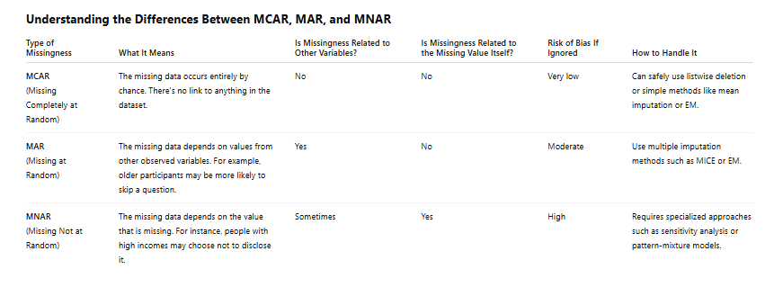
Statistical data preparation: management of missing values and ...
This resource explains the different types of missing data and the common methods for handling them.
Review the section on missing data types (MCAR, MAR, NMAR). Then, read the overview of handling methods, including complete case analysis and imputation.
Your Task (Part 3):
- Based on the contextual note ("...the stylist prioritized rating all the lace pieces first..."), classify the missing score for Piece #10 as MCAR, MAR, or MNAR. Provide a one-sentence justification.
- Choose a method for handling this missing value. The most common options here are:
- Complete Case Analysis (Deletion): Remove Piece #10 from the dataset.
- Mean/Median/Mode Imputation: Replace the missing value with the mean, median, or mode of a relevant group.
- Justify your choice. Explain why it is appropriate given your classification and the goals of the analysis.
Click to see the solution for Part 3
-
Classification: This is Missing at Random (MAR).
- Justification: The probability of the
Appeal_Scorebeing missing depends on an observed variable in the dataset, which is theFabrictype (the stylist prioritized 'Lace' over 'Satin').
- Justification: The probability of the
-
Choice and Justification:
- Method: Imputation using the mean score of a relevant subgroup.
- Justification: Since the data is MAR, simply deleting the row (complete case analysis) would systematically remove a satin piece, potentially biasing our future analysis against satin fabric. A better approach is to impute a reasonable value. A good strategy is to use the average score of similar items. Here, we can impute the mean score of the other 'Balconette' style pieces.
- The other balconettes are Piece #2 (Score: 8) and Piece #6 (Score: 9). The mean is . We will impute
8.5for Piece #10.
Final Step: Assembling the Clean Dataset
You have now made justified decisions for every problematic data point. The final step is to apply these changes and create the clean dataset that will serve as the foundation for all subsequent analyses in this project.
Your Task (Part 4):
- Create the final, cleaned list of 12
Appeal_Scorevalues, incorporating your decisions from the outlier and missing value steps.
Click to see the final cleaned dataset
Here is the original list of scores with issues highlighted:9, 8, 7, 10, 2, 9, 6, **1**, 8, **NULL**, 7, 8
- Outlier Handling: The score of
1(Piece #8) is Winsorized to2. - Missing Value Handling: The
NULLscore (Piece #10) is imputed with8.5.
Final Cleaned Appeal_Score list:9, 8, 7, 10, 2, 9, 6, **2**, 8, **8.5**, 7, 8
Conclusion
In this capstone lesson for Module 1, you have navigated the essential first step of any data analysis project: data cleaning and preparation. By systematically identifying, classifying, and addressing both outliers and missing values, you have transformed a raw, potentially misleading dataset into a robust foundation for analysis.
Key Takeaways:
- Data cleaning is not just a mechanical process; it requires critical thinking and justification at every step.
- The choice of how to handle outliers (trimming vs. Winsorizing) and missing values (deletion vs. imputation) depends on the underlying reason for the issue (error vs. true value, MCAR vs. MAR vs. MNAR).
- Your decisions should always be made with the final analytical goal in mind—in this case, gaining clear and unbiased insights into what drives a lingerie piece's photogenic appeal.
With your clean dataset in hand, you are now ready to move from preparation to discovery. In the next module, "Identifying Trends and Style Relationships," we will begin to explore the patterns in this data, starting with one of the most fundamental statistical tools: correlation.