Welcome to the next stage of our data analysis journey. In our previous lessons, we built a solid foundation by developing skills to clean and prepare your lingerie rating dataset. You learned to manage missing data by understanding its underlying mechanism and to robustly detect and handle outliers using the IQR method. With a clean dataset, you are now ready to move from preparation to exploration.
This lesson focuses on the heart of exploratory data analysis (EDA): using summary statistics and visualizations to uncover the initial stories hidden within your data. Our goal is to analyze your dataset of lingerie attributes and ratings to generate the first set of testable hypotheses about what design features drive appeal. This is the crucial creative step where you begin to translate raw numbers into design insights for your photoshoot project.
From Raw Numbers to Initial Insights: Summary Statistics
Before we create a single chart, we can learn a great deal by summarizing our data numerically. Given your background in statistics, you are well-acquainted with these measures, so our focus will be squarely on their application and interpretation in the context of lingerie design.
We'll consider two main types of variables in your dataset:
-
Categorical Variables: These describe qualitative attributes like
Style('push-up', 'balconette', 'bralette'),Fabric('lace', 'satin', 'mesh'), orColor('red', 'black', 'nude').- The primary tool here is the frequency distribution. By calculating counts and percentages, you can quickly identify the dominant characteristics in your dataset. For example, if you analyze a collection of top-rated lingerie pieces and find that 70% are made of 'lace', this forms an immediate hypothesis: "Lace is a key driver of high ratings."
-
Numerical Variables: These are quantitative measurements like
Appeal Rating(1-10),Neckline Depth(in cm), orStrap Width(in mm).- Measures of Central Tendency (Mean vs. Median): As we discussed in the outlier lesson, the mean gives the average rating, while the median gives the middle rating. If the mean appeal score for a balconette bra is significantly lower than its median, it suggests the presence of a few very low scores (negative outliers) that are pulling the average down. This might indicate an issue with fit for certain body types, rather than a universally disliked design.
- Measures of Dispersion (Standard Deviation and IQR): A low standard deviation in the ratings for a particular style (e.g., a simple bralette) implies a consensus; most people feel similarly about it. Conversely, a high standard deviation for a more daring piece (e.g., a strappy cupless bra) might indicate it's a polarizing design—loved by some, disliked by others. This is a crucial insight for a photoshoot, where a polarizing but striking look can be more effective than a universally "okay" one.
Visualizing the Story: Key Chart Types
While summary statistics are powerful, visualizations are essential for revealing patterns that numbers alone cannot. We will explore four key visualization types to help you build hypotheses about your lingerie designs. The following resource provides a good overview of the most common charts.
3 Basic Data Visualizations – Introduction to Statistics - Bookdown
This table provides a quick reference for several common chart types, their uses, and their pros and cons.
Please review the summary Table 3.1 at the end of the chapter. Pay attention to the "Use_Case" column to see how each chart type aligns with different analytical questions.
Now, let's dive into how to apply these charts to your lingerie dataset.
1. How is an attribute distributed? The Histogram
The first question you might ask is about the nature of a single numerical attribute. For instance, what do the appeal ratings across all your pieces look like? Are most of them high? Is there a wide spread?
A histogram is the perfect tool for this. It groups numerical data into bins and plots the frequency of each bin, revealing the shape of the distribution.
3 Basic Data Visualizations – Introduction to Statistics - Bookdown
This section explains what a histogram is and how it visualizes the distribution of numerical data.
Read the section on Histograms to understand its purpose. You can skim the code examples, as our focus is on interpretation.
Imagine you create a histogram of appeal ratings for 50 lingerie pieces.
- A skew to the right (a long tail of high ratings) suggests most pieces are rated highly, which is a good sign.
- A bimodal distribution (two distinct peaks) could be very insightful. It might indicate that your raters fall into two groups with different tastes, or that the lingerie pieces themselves belong to two distinct clusters of appeal (e.g., 'everyday comfort' vs. 'glamour photoshoot'). This would be a hypothesis worth investigating further.
2. How do different styles compare? The Box Plot
Your most pressing question is likely: "Which lingerie styles perform best?" To answer this, you need to compare a numerical variable (Appeal Rating) across a categorical variable (Style). Bar charts are often used for this, showing the mean rating for each category.

The bar charts in the image above effectively compare the average rating across different product groups. However, they hide the distribution. A far more informative tool is the box plot, which you are already familiar with from our lesson on outliers.
3 Basic Data Visualizations – Introduction to Statistics - Bookdown
This section provides a detailed look at box plots and how they are used to compare distributions across groups.
Read the main description in section 3.6 Box-plot. Then, look at the final example chart in the section (Figure 3.12), which compares "Total Price" across different "Product Categories". This is directly analogous to comparing Appeal Rating across Lingerie Style.
By placing box plots for 'Push-up', 'Balconette', and 'Bralette' side-by-side, you can generate powerful hypotheses:
- Comparing Medians: Does the median line for 'Balconette' sit higher than for 'Push-up'? Hypothesis: "Balconettes are generally rated higher."
- Comparing Box Sizes (IQR): Is the box for 'Bralette' much taller than for 'Balconette'? Hypothesis: "There is less consensus on the appeal of bralettes; their ratings are more variable."
- Observing Outliers: Does the 'Push-up' category have several low-rating outliers? Hypothesis: "Push-up bras may have fit issues for some models, leading to exceptionally low scores."
3. What is the relationship between numerical attributes? The Scatter Plot
You might also wonder if two numerical features are related. For instance, does a deeper plunge neckline lead to a higher appeal score? Or is there a trade-off between the percentage of lace coverage and perceived comfort? The scatter plot is the classic tool for this.
3 Basic Data Visualizations – Introduction to Statistics - Bookdown
This section introduces the scatter plot for visualizing the relationship between two continuous variables.
Read the description under section 3.7 Scatter-plot. Focus on the types of patterns it can reveal: trends, correlations, and clusters.
By plotting Neckline Depth on the x-axis and Appeal Rating on the y-axis, you could hypothesize:
- A positive linear trend: "As neckline depth increases, appeal rating tends to increase."
- A non-linear (curved) trend: "Appeal rating increases with neckline depth up to a point, after which it plateaus or declines." This would be a critical insight for design optimization.
- No clear pattern: "Neckline depth does not appear to be a significant driver of appeal."
4. How do categorical attributes interact? The Heatmap
Finally, you may want to understand the relationship between two categorical variables. For example, which Styles are most recommended within different Price categories? A heatmap is a fantastic way to visualize this interaction. It uses color intensity to represent values in a matrix.
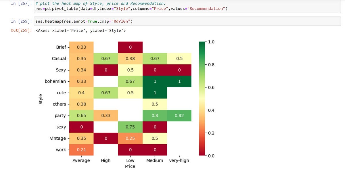
Let's interpret the heatmap above to generate hypotheses:
- Looking at the 'bohemian' row, we see high recommendation scores (green) only in the 'Medium' and 'very-high' price columns. Hypothesis: "Bohemian styles are perceived as suitable only for mid-to-high price points, but not for low or high."
- The 'sexy' style has a value of 0 for 'Average' price but a high value of 0.75 for 'Low' price. Hypothesis: "The 'sexy' label is applied differently across price points, with a strong association in the 'Low' category but none in the 'Average' one."
- The bright green cells for
cuteandbohemianstyles under 'Medium' and 'very-high' price suggest a strong positive association. Hypothesis: "These styles are the top performers in these specific price segments."
Numerical Exercise
You have collected data for 5 new lingerie pieces you've designed. Your dataset looks like this:
| Piece ID | Style | Fabric | Lace Coverage (%) | Appeal Rating (1-10) |
|---|---|---|---|---|
| 1 | Bralette | Lace | 80 | 9 |
| 2 | Balconette | Satin | 20 | 8 |
| 3 | Bralette | Mesh | 50 | 6 |
| 4 | Balconette | Lace | 60 | 9 |
| 5 | Bralette | Lace | 90 | 5 |
Your Task:
- Calculate the summary statistics for
Appeal Ratingfor eachStyle(Bralette vs. Balconette). What is the mean and median rating for each? - Based on your statistics, what is your initial hypothesis about which style is performing better?
- Describe what a histogram for
Lace Coverage (%)would look like based on this data. What does it tell you about your collection of 5 pieces? - Based on a visual inspection of the table, state one hypothesis about the relationship between
Lace Coverage (%)andAppeal Rating. What kind of plot would you use to investigate this?
Conclusion
In this lesson, we transitioned from data cleaning to data exploration. You've learned how to leverage your existing statistical knowledge to interpret summary statistics and key visualizations—histograms, box plots, scatter plots, and heatmaps—in the specific context of lingerie design. This process is the foundation for developing data-driven insights.
Key Takeaways:
- Exploratory Data Analysis (EDA) is about asking questions of your data to generate hypotheses.
- Summary statistics (mean, median, standard deviation) provide a quick numerical overview, but their interpretation depends on the context of your design goals.
- Histograms reveal the distribution of a single numerical attribute.
- Box plots are excellent for comparing distributions across different categories (e.g., ratings across styles).
- Scatter plots help uncover relationships between two numerical attributes.
- Heatmaps visualize the interaction between two categorical attributes.
You are now equipped with the fundamental tools for the first phase of your project: Trend Analysis. In our next and final lesson of this module, we will put everything together. You will tackle a comprehensive numerical problem that requires you to clean a small dataset with both missing values and outliers and then perform a brief exploratory analysis to justify your decisions and state your initial findings.