Back-Door Criterion for Causal Inference in Lingerie Photoshoots

Welcome back. In our previous lesson, we learned to map out the causal relationships in a lingerie photoshoot using Directed Acyclic Graphs (DAGs). We identified the three basic building blocks—chains, forks, and colliders—and saw how a "fork" structure, or confounder, creates a non-causal "backdoor path" between our treatment and outcome. This gave us a visual language for the problem we first encountered with Simpson's paradox.

Today, we move from diagnosis to treatment. Knowing that backdoor paths exist is one thing; knowing precisely how to block them is another. This lesson introduces the back-door criterion, a rigorous, graph-based rule that tells you exactly which variables you must control for (or "condition on") to isolate the true causal effect of a lingerie style on photoshoot ratings. This will equip you with a formal method to design a statistically valid analysis and avoid drawing spurious conclusions.

Backdoor Paths and the Goal of Adjustment

Let's quickly formalize what we mean by a "backdoor path." A backdoor path is a non-causal path between a treatment (D) and an outcome (Y) that begins with an arrow pointing into the treatment.

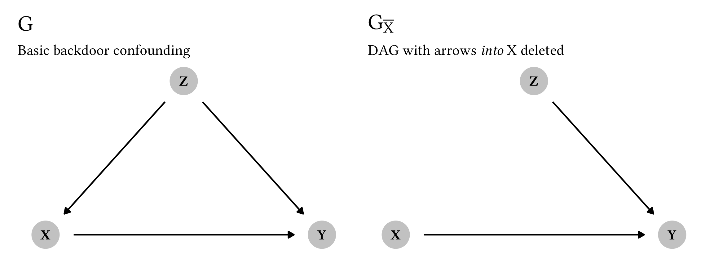
The graph on the left, G, shows a simple DAG where Z is a confounder creating a backdoor path X ← Z → Y. The graph on the right, G_x-bar, represents the conceptual goal of causal inference: to estimate the effect of X on Y as if the influence of confounders on X were removed.

In our running example, Lingerie Style (X) ← Model Body Type (Z) → Photoshoot Rating (Y), the path via Model Body Type is a backdoor path. It's a source of spurious correlation because Model Body Type influences both which style is chosen and the final rating. Our goal is to "block" or "close" this path, leaving only the direct causal arrow X → Y to be estimated. The back-door criterion is our rulebook for doing this correctly.

The Back-Door Criterion: A Formal Rule

To estimate the causal effect of a treatment D on an outcome Y, we need to find a set of variables, let's call it Z, to control for in our analysis. The back-door criterion tells us whether a proposed set Z is "sufficient" to close all confounding pathways.

A set of variables Z satisfies the back-door criterion relative to an ordered pair of variables (D, Y) in a DAG if:

No node in Z is a descendant of D (i.e., you don't control for variables that are caused by the treatment).
Z blocks every path between D and Y that contains an arrow into D (i.e., Z closes all backdoor paths).

This might seem abstract, so let's break down rule #2. A path is blocked by a set Z if either:

The path contains a chain (A → M → B) or a fork (A ← C → B) where the middle variable (M or C) is in the set Z.
The path contains a collider (A → C ← B) where the collider C is NOT in the set Z, and no descendant of C is in Z.

This leads to a simple, two-part strategy for closing backdoor paths:

Condition on confounders: Find the common causes that create backdoor forks and include them in your model.
Do NOT condition on colliders: Colliders naturally block paths. Conditioning on them opens the path, introducing bias.

The following reading from Scott Cunningham's Causal Inference: The Mixtape provides an excellent, formal walkthrough of these concepts.

3 Directed Acyclic Graphs – <span style='font-weight

This chapter clearly defines backdoor paths, explains the special role of colliders, and formally states the back-door criterion.

First, read the introduction to backdoor paths, starting from the description of a simple DAG. Then, read the section defining a collider and its unique properties. Finally, focus on the section defining the backdoor criterion itself. This provides the formal rules for how to close a backdoor path by conditioning.

Finding the Adjustment Set: A Lingerie Photoshoot Example

Let's apply this to the DAG we developed in the previous lesson. Our goal is to find the causal effect of Lingerie Style (T) on Photoshoot Rating (Y).

A complex DAG illustrating various causal paths in a photoshoot. Here we relabel the nodes for our context: T=Lingerie Style, Y=Photoshoot Rating, Z=Model Body Type, W=Stylist's Expertise, X=Selected for Final Edit, Ut/Uz/Ux/Uy/Uu/Uw=Unobserved factors.

Let's adapt this general graph to our specific variables from last lesson for clarity:

T: Lingerie Style
Y: Photoshoot Rating
Z: Model Body Type
W: Model Confidence
X: Selected for Final Edit

Let's trace the key paths from T to Y and decide what to do with them:

Path 1: T → Y
- Type: Direct causal path.
- Action: This is the effect we want to estimate. We must leave this path open.
Path 2: T → W → Y (i.e., Lingerie Style → Model Confidence → Photoshoot Rating)
- Type: A causal path mediated by Model Confidence.
- Action: If we want the total causal effect of the style, we must leave this path open. Conditioning on the mediator W would block this path and give us only the direct effect of T on Y, which is a different research question. So, we do not condition on W.
Path 3: T ← Z → Y (i.e., Lingerie Style ← Model Body Type → Photoshoot Rating)
- Type: A classic backdoor path with Z as a confounder (a fork).
- Action: This path is open and introduces bias. To block it, we must condition on the confounder Z.
Path 4: T → X ← Y (i.e., Lingerie Style → Selected for Final Edit ← Photoshoot Rating)
- Type: This path contains a collider, X.
- Action: The path is naturally blocked by the collider. To keep it blocked, we must not condition on X. Analyzing only the styles that were selected for the final edit would be conditioning on this collider and would introduce collider bias.

Conclusion:
To estimate the total causal effect of Lingerie Style on Photoshoot Rating, the correct adjustment set is {Model Body Type}. We must control for Model Body Type but must not control for Model Confidence or Selected for Final Edit.

Automating the Search with R

Given your background in statistics and R, you'll appreciate that this entire process can be automated. Manually listing paths is feasible for simple DAGs, but for complex ones, software is essential. The dagitty package in R is the standard tool for this.

The key function is adjustmentSets(), which takes a DAG object and returns all valid (minimal) sets of variables that satisfy the back-door criterion.

The following tutorial shows exactly how to use this function.

The Backdoor Criterion and Basics of Regression in R | | Tutorials

This tutorial demonstrates how to use the dagitty::adjustmentSets() function in R to automatically find the correct set of variables to control for.

Focus on the subsection titled "Covariate adjustment". The example shows how to define a DAG and then pass it to dagitty::adjustmentSets() to find the required controls.

This programmatic approach removes guesswork and ensures you have a valid research design, provided your causal assumptions encoded in the DAG are correct.

Your Turn: Numerical Exercise

Now, let's apply these principles to a new scenario. Your task is to identify the correct adjustment set based on a causal story.

Scenario:
You want to estimate the causal effect of Lace Content (as a percentage, T) on a lingerie piece's Aesthetic Score (Y). Your causal assumptions are:

Lace Content (T) directly affects the Aesthetic Score (Y).
The Garment Type (Z1, e.g., bra vs. panty) influences the typical Lace Content and also independently affects the Aesthetic Score.
The Garment Type (Z1) also determines the required Garment Complexity (M, e.g., number of panels), and this Complexity in turn affects the Aesthetic Score.
The overall Brand Collection (Z2, e.g., 'Bridal' vs. 'Everyday') influences both the Garment Type chosen and the target Aesthetic Score.
Finally, to create a curated portfolio, only pieces with a high Aesthetic Score (Y) or a very high Lace Content (T) are selected for a special "Premium" Label (C).

Your Task:

Based on the story, list the causal relationships.
Draw the corresponding DAG.
List all paths (causal and non-causal) from Lace Content (T) to Aesthetic Score (Y).
For each path, identify its type (causal, backdoor, or blocked by collider).
Determine the minimal sufficient adjustment set(s) to estimate the total causal effect of T on Y. Justify your choices.

Click for the solution.

1. Causal Relationships:

T → Y
Z1 → T
Z1 → Y
Z1 → M
M → Y
Z2 → Z1
Z2 → Y
T → C
Y → C

2. DAG:

A possible DAG for this scenario would show arrows representing the relationships above. The key features are:

Z1 and Z2 are confounders.
M is a mediator of Z1's effect, but not on the T->Y path.
C is a collider.

3. Paths from T to Y:

Path 1: T → Y (Direct causal)
Path 2: T ← Z1 → Y (Backdoor)
Path 3: T ← Z1 ← Z2 → Y (Backdoor)
Path 4: T ← Z1 → M → Y (Backdoor)
Path 5: T → C ← Y (Blocked by collider)

4. Path Analysis:

Path 1 (T → Y): Causal. Must remain open.
Path 2 (T ← Z1 → Y): Open backdoor path via the confounder Z1. Must be blocked.
Path 3 (T ← Z1 ← Z2 → Y): Open backdoor path via the confounder Z2. Must be blocked.
Path 4 (T ← Z1 → M → Y): Open backdoor path. Must be blocked.
Path 5 (T → C ← Y): Path is naturally blocked by the collider C. Must remain blocked.

5. Minimal Sufficient Adjustment Set:

To block all open backdoor paths, we need to choose a set of variables.

Conditioning on {Z1} blocks Path 2 and Path 4. It also blocks Path 3, as the path T ← Z1 ← Z2 is now blocked at Z1.
Conditioning on {Z2} alone is not enough, as Path 2 and Path 4 remain open.
We must not condition on the collider C.
The variable M is not on a backdoor path from T to Y, but it is on a backdoor path from T to Y via Z1. Controlling for Z1 already closes this path.

Therefore, the single minimal sufficient adjustment set is {Garment Type (Z1)}. Controlling for Garment Type is sufficient to block all confounding between Lace Content and Aesthetic Score in this model. Another valid, though not minimal, set would be {Z1, Z2}.

Conclusion

In this lesson, we formalized the process of identifying and blocking confounding pathways using the back-door criterion. This powerful tool, grounded in the causal structure of your DAG, provides a definitive method for selecting control variables.

Key Takeaways:

The Goal of Adjustment: To block all non-causal backdoor paths between the treatment and outcome.
The Back-Door Criterion: A set of variables Z is a valid adjustment set if it doesn't contain any descendants of the treatment and it blocks all backdoor paths.
Practical Strategy: Achieve this by conditioning on confounders (forks/chains on backdoor paths) while strictly avoiding conditioning on colliders or mediators on the causal path of interest.
Automation: Tools like the dagitty package in R can automatically identify valid adjustment sets, making this process robust and scalable.

We've emphasized the danger of conditioning on a collider. In our next lesson, we will explore this issue in more depth by examining Berkson's paradox, a fascinating and common form of collider bias that can arise from sample selection—for example, by analyzing only the lingerie pieces that were ultimately chosen for a photoshoot.