In our last session, we established the back-door criterion as a formal rule for deciding which variables to control for to isolate a causal effect. This powerful technique helps us block confounding paths. However, we also issued a crucial warning: never condition on a collider. Today, we delve into the "why" behind that warning by exploring a famous statistical pitfall known as Berkson's paradox.
This lesson will demonstrate how conditioning on a collider, a common effect of two other variables, doesn't just fail to help—it actively creates spurious associations. We'll see how this paradox can manifest in your work, for instance, by creating a false trade-off between two desirable lingerie attributes simply because of how you select your final pieces for a photoshoot. This is the final piece of the puzzle you need to correctly apply causal reasoning and avoid being misled by your own data.
The Anatomy of Collider Bias
Let's begin by visually recalling the difference between a confounder (which we learned to control for) and a collider (which we must not).
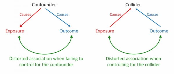
In the previous lesson, we focused on closing the "backdoor path" created by a confounder. Today, our focus is on the right-hand diagram. A collider is a variable that is a common effect of two other variables. In the diagram, both "Exposure" and "Outcome" are causes of the "Collider". The path Exposure → Collider ← Outcome is naturally blocked at the collider. However, if you condition on the collider—by filtering, stratifying, or controlling for it in a regression—you open this path, creating a non-causal association between the Exposure and the Outcome. This induced association is what we call collider bias, or Berkson's paradox.
To make this tangible, consider two attributes of lingerie designs that are, for the sake of argument, completely independent in the general population of all possible designs: Aesthetic Appeal and Wearable Comfort. Now, imagine your selection process for the final photoshoot. You create a "final consideration" pool. A lingerie piece makes it into this pool only if it meets a certain threshold of overall quality. This means it must be either very aesthetically appealing, very comfortable, or have a good combination of both.
Selected for Final Shoot is your collider. It is caused by both Aesthetic Appeal and Wearable Comfort.
Aesthetic Appeal → Selected for Final Shoot ← Wearable Comfort
Now, if you only analyze the pieces within this selected pool, a strange thing happens. If you pick a piece from this pool and find it is not very comfortable, you can infer it must be highly aesthetic to have made the cut. Conversely, a selected piece that isn't visually stunning must be exceptionally comfortable. This creates a spurious negative correlation between comfort and aesthetics in your selected sample, even if no such trade-off exists in the wider world of lingerie design. This is Berkson's paradox in action.

The following article provides a clear definition of the paradox and some classic examples that will help solidify your intuition.
Berkson's Paradox Explained: Why Selection Bias Creates False ...
This article defines Berkson's Paradox, explains its mechanism as collider bias, and provides several relatable examples.
Please read the first section, "What Is Berkson's Paradox?", for a formal definition and a brief mathematical intuition. Then, read the section on the dating market paradox, which is a perfect analogy for the Aesthetic Appeal vs. Comfort example we just discussed.
A Deeper Dive: Simulation and Selection Effects
Given your statistics background, we can explore this phenomenon with more rigor. The intuition is useful, but a quantitative model reveals just how potent and counterintuitive collider bias can be. We'll examine a simulation-based analysis that investigates a similar problem in job hiring.
Let's translate the hiring example from the reading into our lingerie context. Suppose the ultimate Photoshoot Success of a lingerie piece is determined by two independent factors:
- Technical Virtuosity (T): The complexity and quality of the garment's construction (e.g., intricate lace patterns, advanced boning).
- Stylistic Flair (O): Other, less tangible factors like how well it matches the model's personality, the current trendiness, etc.
Both T and O contribute positively to Photoshoot Success. Now, the selection process for which pieces get used in the shoot is a collider. A stylist might create a composite score based on a weighted combination of T and O to decide what to include.
The fascinating discovery from the simulation is that if the selection process becomes very stringent and slightly over-weights Technical Virtuosity (T), the relationship between T and Photoshoot Success can appear to be zero or even negative among the selected pieces. This means that within the elite group of lingerie chosen for the shoot, it might look like the most technically complex pieces perform worse, even though in reality, technical skill is a strong positive driver of success.
This happens because an over-reliance on T in the selection process means that pieces with extremely high T scores can get selected even if their Stylistic Flair (O) is mediocre. Conversely, pieces with moderate T scores must have exceptionally high O scores to make the cut. This "explaining away" effect, induced by conditioning on the collider, distorts the true relationship.
The following resource provides a brilliant walk-through of this simulation. While the code is in Python, the logic and statistical concepts are universal and will be clear to you.
An analysis of Berkson's Paradox - Of Aurochs and Angels
This blog post provides an in-depth simulation of Berkson's paradox in a selection context, which we can apply directly to our lingerie photoshoot scenario.
Start by reading the setup in section 2, focusing on the description of the model. This sets up the causal structure with "Got Hired" as the collider. Then, review section 5, which presents the core results. Pay close attention to the graph plotting the effect size against the selection weighting, and the author's explanation of the "negative effect size well". Finally, read section 6, which contains a critical discussion on why focusing on effect size is often more insightful than using correlation, especially when variance is restricted by selection—a nuance that is highly relevant in applied statistical work.
The key insight is that your analysis can be dangerously misleading if you only look at your "winners." A naive analysis of only the lingerie that made it into the final photoshoot might lead you to incorrectly conclude that a certain desirable attribute (like Technical Virtuosity) is unimportant or even detrimental to success. The paradox teaches us that this apparent negative effect could be a pure artifact of your selection process.
Your Turn: Demonstrating the Paradox
Let's prove this to ourselves with a numerical exercise.
Scenario:
You're evaluating 20 potential lingerie pieces for a boudoir photoshoot. From past experience, you know that a piece's suitability is driven by two independent factors: Visual Impact (VI) and Model Comfort (MC), both rated on a scale of 1 to 10. For this exercise, we will assume they are roughly uncorrelated in the general population of designs.
A piece is selected for the "final consideration set" if the sum of its scores (VI + MC) is 15 or greater.
Data:
Here are the scores for the 20 pieces:
| Piece ID | Visual Impact (VI) | Model Comfort (MC) |
|---|---|---|
| 1 | 7 | 4 |
| 2 | 10 | 8 |
| 3 | 4 | 2 |
| 4 | 1 | 7 |
| 5 | 8 | 8 |
| 6 | 10 | 6 |
| 7 | 8 | 1 |
| 8 | 4 | 5 |
| 9 | 9 | 7 |
| 10 | 2 | 8 |
| 11 | 8 | 5 |
| 12 | 9 | 9 |
| 13 | 10 | 3 |
| 14 | 2 | 3 |
| 15 | 1 | 2 |
| 16 | 6 | 4 |
| 17 | 10 | 3 |
| 18 | 6 | 9 |
| 19 | 1 | 4 |
| 20 | 5 | 1 |
Your Task:
- Calculate the Pearson correlation coefficient between
Visual Impact(VI) andModel Comfort(MC) for the entire dataset of 20 pieces. - Create a "selected subset" by identifying all pieces where
VI + MC ≥ 15. - Calculate the Pearson correlation coefficient between VI and MC for this selected subset.
- Explain the difference between the two correlation coefficients using the concept of Berkson's paradox.
Click for the solution.
1. Correlation for the Entire Dataset:
First, we calculate the correlation for all 20 pieces. Using statistical software or a calculator on the full dataset:
- The Pearson correlation coefficient between VI and MC is approximately -0.126.
- This value is very close to zero, confirming our initial assumption that
Visual ImpactandModel Comfortare largely independent in this general population of designs.
2. Identifying the Selected Subset:
We apply the selection rule VI + MC ≥ 15. The pieces that meet this criterion are:
- Piece 2: 10 + 8 = 18
- Piece 5: 8 + 8 = 16
- Piece 6: 10 + 6 = 16
- Piece 9: 9 + 7 = 16
- Piece 12: 9 + 9 = 18
- Piece 18: 6 + 9 = 15
This gives us a selected subset of 6 pieces.
3. Correlation for the Selected Subset:
Now, we calculate the correlation only for these 6 selected pieces:
| Piece ID | Visual Impact (VI) | Model Comfort (MC) |
|---|---|---|
| 2 | 10 | 8 |
| 5 | 8 | 8 |
| 6 | 10 | 6 |
| 9 | 9 | 7 |
| 12 | 9 | 9 |
| 18 | 6 | 9 |
- The Pearson correlation coefficient for this subset is approximately -0.743.
4. Explanation:
The correlation dramatically changed from near-zero (-0.126) in the full population to strongly negative (-0.743) in the selected sample. This is a classic demonstration of Berkson's paradox.
- The selection criterion (
VI + MC ≥ 15) acts as a collider. Both highVisual Impactand highModel Comfortincrease the chances of being selected. - By filtering our data to include only the selected pieces, we are conditioning on this collider.
- This conditioning opens a spurious path between VI and MC. Within this elite group, a piece with a lower VI score (like Piece 18 with VI=6) must have a high MC score (MC=9) to have been selected. Conversely, a piece with a lower MC score (like Piece 6 with MC=6) must compensate with a high VI score (VI=10).
- This creates the illusion of a trade-off, or a negative correlation, between Visual Impact and Model Comfort that does not exist in the general population of designs. An analyst looking only at the "finalists" would wrongly conclude that beautiful lingerie is rarely comfortable.
Conclusion
In this lesson, we explored the significant risks of collider bias through the lens of Berkson's paradox. You now have a clear understanding of not just that you shouldn't condition on colliders, but why it's so problematic.
Key Takeaways:
- Berkson's Paradox is a form of selection bias where conditioning on a common effect (a collider) creates a spurious correlation between its causes.
- In practice, this means that analyzing only a "successful" subset of your data (e.g., lingerie in the final shoot, top-selling items, highly-rated designs) can lead to false conclusions about the relationships between attributes.
- The paradox can create the illusion of a negative trade-off between two desirable qualities (like comfort and beauty) where none exists in the broader population.
- Using causal DAGs to identify colliders before analysis is your primary defense against this subtle but powerful bias.
In our final lesson of this module, we will bring everything together. We will revisit Simpson's paradox, armed with our new knowledge of DAGs and adjustment criteria, and work through a numerical problem to apply a formal adjustment strategy and recover the true causal effect from confounded data.