In our last lesson, we constructed a decision tree using the CART algorithm, guided by the Gini index to make the most informative splits. You saw how this method creates a clear, rule-based flowchart for classifying lingerie styles. This approach is powerful, but it's not the only way to build a decision tree.
Today, we'll explore a prominent alternative: the C4.5 algorithm. Our focus will be on comparing the structure of a tree built with C4.5 to the CART tree from our previous lesson. The core difference lies in the splitting criterion. Instead of Gini impurity, C4.5 uses a concept from information theory called Information Gain, which is based on entropy. By understanding this alternative, you'll gain a more nuanced view of how different algorithms can interpret the same dataset to find predictive patterns.
A Different Measure of Purity: Entropy
In the last lesson, we used the Gini index to measure the "impurity" of a node. A pure node (all 'Photoshoot-Worthy' or all 'Not Worthy') had a Gini index of 0. The C4.5 algorithm, and its predecessor ID3, use a similar concept called Entropy.
In information theory, entropy is a measure of the uncertainty or unpredictability in a system. For our purposes, it quantifies the impurity of a set of examples.
- A perfectly pure node has an entropy of 0 (no uncertainty).
- A node with a 50/50 split of two classes has an entropy of 1 (maximum uncertainty).
The algorithm's goal, much like with the Gini index, is to make splits that reduce uncertainty. The measure of this reduction is called Information Gain. A split with higher information gain is considered better because it reduces our uncertainty about the outcome more significantly.
The following reading explains the formulas for Entropy and Information Gain. Given your statistics background, you may already be familiar with the concept of entropy; this will formalize its application in decision trees.
Chapter 1 Classification and Regression Trees (CART)
This document covers the mathematical foundations of various tree algorithms. We will focus on the sections defining Entropy and Information Gain.
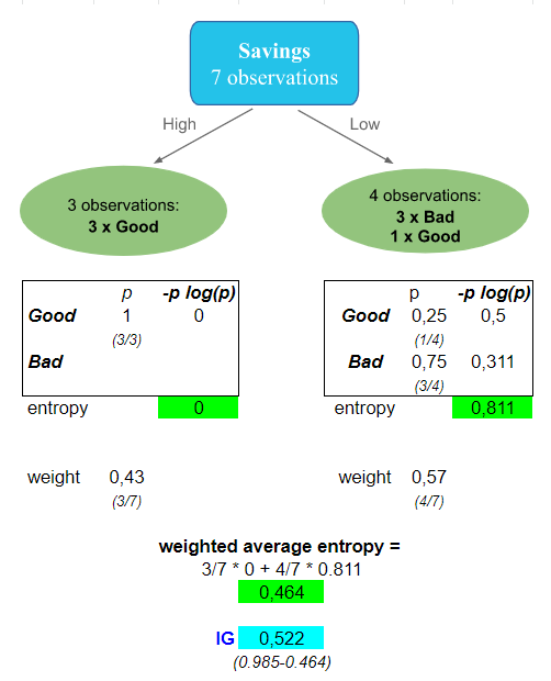
Please start at the section "Splitting Criterion & Best Split." Briefly review the Gini Impurity formula to refresh your memory. Then, focus on the definitions provided for Entropy and Information gain. Note the formula for entropy, H(S) = -\sum p(x)\log_2 p(x), and how information gain, IG(A,S), is simply the entropy of the parent node minus the weighted average entropy of the child nodes.
To visualize this calculation, let's look at a simple example.
CART vs. C4.5: Key Structural and Algorithmic Differences
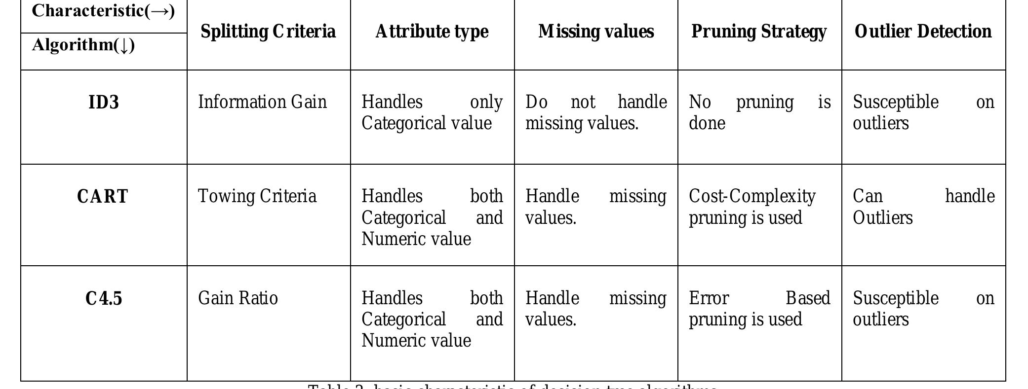
While both CART and C4.5 aim to create rule-based classifiers, their different splitting criteria and mechanics can lead to trees with notably different structures. Here are the most important distinctions:
-
Splitting Criterion: As we've discussed, CART uses the Gini Index, while C4.5 uses Information Gain. While they often lead to similar splits, they can diverge, especially when one split creates a perfectly pure node while another makes both child nodes "pretty good."
-
Tree Structure (Binary vs. Multi-way Splits): This is a critical structural difference. CART always creates binary trees, where each node has exactly two branches (e.g.,
Color Tone = Darkvs.Color Tone != Dark). In contrast, C4.5 can create multi-way splits for categorical attributes. For an attribute likeFabric = {Lace, Satin, Cotton}, a C4.5 tree could have a single node with three branches, one for each fabric type. This can lead to shorter, wider trees compared to the taller, binary trees of CART. -
Refinement for Attribute Selection (Gain Ratio): A known issue with Information Gain is its bias towards attributes with many unique values (e.g., a
Style_IDfeature would have maximum information gain but is useless for generalization). To counteract this, C4.5 uses a normalized version called Gain Ratio. It penalizes attributes with many outcomes by dividing the Information Gain by the attribute's own intrinsic entropy. This leads to more robust feature selection. -
Other Differences: The algorithms also differ in how they handle missing values and how they prune the tree to prevent overfitting, but the splitting criterion and tree structure are the most fundamental points of comparison.
The following table neatly summarizes these differences.
For a more detailed textual summary of these points, you can consult the following resources.
Chapter 1 Classification and Regression Trees (CART)
This section of the "Classification and Regression Trees" document provides a direct, bulleted comparison of the two algorithms.
Read the short list under the heading "CART vs C4.5" to reinforce the key differences we just discussed.
[PDF] Comparative Study Id3, Cart And C4.5 Decision Tree Algorithm
This survey paper offers concise definitions and comparisons. It's particularly useful for its explanation of Gain Ratio.
In section III, "SPLITTING CRITERIA", find the definition for Gain Ratio. This explains the normalization C4.5 uses. Then, in section IV, under "C4.5", read the description of how it handles attributes.
Your Turn: Comparing Splits on the Lingerie Dataset
Now, let's put theory into practice. We will use the exact same dataset from our CART exercise in the previous lesson. Your task is to calculate the Information Gain for each feature to determine which split the C4.5 algorithm would choose.
Recall the Dataset:
| Style ID | Has Lace? | Support | Color Tone | Photoshoot-Worthy |
|---|---|---|---|---|
| 1 | Yes | Low | Dark | Yes |
| 2 | No | High | Dark | Yes |
| 3 | No | Low | Light | No |
| 4 | Yes | High | Dark | Yes |
| 5 | No | Low | Dark | No |
| 6 | No | High | Light | No |
| 7 | Yes | Low | Dark | Yes |
| 8 | No | High | Dark | Yes |
Your Task:
- Calculate the entropy of the root node (the entire dataset).
- For each of the three features (
Has Lace?,Support,Color Tone), calculate the Information Gain of a split. - Identify which feature provides the best split (i.e., the highest Information Gain).
- Compare this result to the one from our previous CART/Gini index exercise. Did both algorithms choose the same feature for the first split?
Hint: Remember that . You'll be working with fractions, and a calculator is recommended.
Click for the step-by-step solution.
1. Entropy of the Root Node
- Total samples: 8
- Photoshoot-Worthy (Yes): 5
- Photoshoot-Worthy (No): 3
- ,
2. Information Gain for Each Feature
a) Feature: Has Lace?
- Lace = Yes (3 samples): {Yes: 3, No: 0}. This node is pure.
- Lace = No (5 samples): {Yes: 2, No: 3}.
- Weighted Entropy:
- Information Gain:
b) Feature: Support
- Support = High (4 samples): {Yes: 3, No: 1}.
- Support = Low (4 samples): {Yes: 1, No: 3}.
- Weighted Entropy:
- Information Gain:
c) Feature: Color Tone
- Tone = Dark (6 samples): {Yes: 5, No: 1}.
- Tone = Light (2 samples): {Yes: 0, No: 2}. This node is pure.
- Weighted Entropy:
- Information Gain:
3. Identify the Best Split
- Information Gain (
Has Lace?): 0.348 - Information Gain (
Support): 0.144 - Information Gain (
Color Tone): 0.4675
The highest Information Gain belongs to the Color Tone feature. This is the best first split according to C4.5/ID3.
4. Comparison with CART
In the previous lesson, we calculated the best split using CART's Gini Index. The results were:
- Weighted Gini (
Has Lace?): 0.3000 - Weighted Gini (
Support): 0.3750 - Weighted Gini (
Color Tone): 0.2085
The CART algorithm also chose Color Tone as the best feature for the first split, as it had the lowest weighted Gini impurity. In this case, both Gini Impurity and Information Gain agreed on the most informative feature to split on. While they often concur, it's not guaranteed. The choice of metric can, and sometimes does, lead to different tree structures, especially deeper in the tree.
Conclusion
In this lesson, we have contrasted the CART and C4.5 decision tree algorithms, focusing on their fundamental difference: the splitting criterion. You have seen how C4.5 uses entropy and information gain to find the most informative splits, and you've confirmed through a numerical exercise that this can sometimes lead to the same conclusions as CART's Gini index.
Key Takeaways:
- C4.5 uses Information Gain (based on entropy) to measure the quality of a split, while CART uses the Gini Index.
- A key structural difference is that C4.5 can create multi-way splits for categorical variables, whereas CART is strictly binary.
- C4.5 improves upon its predecessor (ID3) by using Gain Ratio to prevent a bias towards features with many distinct values.
- The choice of algorithm impacts tree construction and can result in different rule sets, though for many problems, their performance is comparable.
We have now examined two tree-based classifiers and the probabilistic Naive Bayes model. All of these models learn "rules" from the entire training dataset. In our next lesson, we will shift gears to an entirely different classification philosophy: instance-based learning. We'll explore the K-Nearest Neighbors (KNN) algorithm, a model that makes predictions for a new item by simply looking at the classifications of the data points most similar to it.