Welcome to our next lesson. In our previous sessions, we explored classifiers like Naive Bayes and Decision Trees, which learn an explicit model from the training data. For example, a decision tree builds a set of "if-then" rules to make predictions. Today, we shift to a completely different classification philosophy known as instance-based or "lazy" learning.
We will focus on one of the most intuitive algorithms in machine learning: K-Nearest Neighbors (KNN). Instead of building a complex model, KNN classifies a new data point simply by observing the classes of its closest neighbors in the feature space. Your goal for this lesson is to apply a K-Nearest Neighbors model with K=3 to classify a new lingerie piece, using its feature-space neighbors to make the prediction.
The K-Nearest Neighbors Algorithm: Intuition and Process
At its core, KNN operates on a simple principle: you are what your neighbors are. Imagine trying to classify a new, unlabelled lingerie piece that exists in a feature space defined by characteristics like 'structure' and 'delicacy'. The KNN algorithm will find the 'K' most similar, already-labelled lingerie pieces from your dataset and assign the new piece the most common label among them. It's essentially a classification by majority vote.
The entire process can be broken down into four straightforward steps, which are visualized beautifully in the following image.
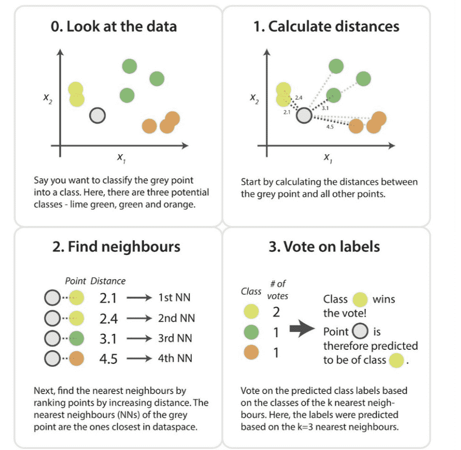
These steps form the complete KNN algorithm. For a more formal description of this process, the following resource provides a concise summary.
Algo Numerical examples (1) (pdf) - CliffsNotes
This document from CliffsNotes outlines the fundamental algorithm for KNN classification.
Read the short section that begins with the inputs and ends with the five steps. Pay close attention to how these steps directly mirror the visual explanation you just saw, particularly the role of 'k' and the distance metric.
The most common distance metric used for continuous features is the Euclidean distance. Given your background in statistics, you'll recognize this as the straight-line distance between two points, and , in an n-dimensional space, calculated as:
A Critical Prerequisite: Feature Scaling
Before applying KNN, there is a crucial data preparation step you must perform: feature scaling. Because KNN relies entirely on distance, features with larger scales can disproportionately dominate the distance calculation.
Imagine you are classifying lingerie based on two features:
Lace Percentage: ranging from 0 to 100.Strap Width (cm): ranging from 0.5 to 2.5.
A difference of 20 in lace percentage would contribute to the squared Euclidean distance, while a large difference of 2 cm in strap width would only contribute . The lace feature would overwhelm the strap width feature, making the model insensitive to its effects.
To prevent this, we must normalize the features so they are on a comparable scale. A common method is Standardization (or Z-score normalization), where you transform each feature to have a mean of 0 and a standard deviation of 1. This ensures all features contribute equally to the distance calculation.
The DataCamp tutorial below explains this concept clearly.
K-Nearest Neighbors (KNN) Classification with scikit-learn
This tutorial walks through building a KNN model and highlights the importance of normalization.
Focus on the section Normalizing & Splitting the Data. The text explains exactly why normalization is essential for a distance-based algorithm like KNN.
Your Turn: Classifying a New Lingerie Style with KNN
Now, let's apply this process. Suppose you have performed PCA on a larger dataset of lingerie attributes and have represented each piece by its score on the first two principal components:
- PC1: 'Structure' (higher values mean more support, underwire, etc.)
- PC2: 'Delicacy' (higher values mean more lace, sheer fabrics, intricate details)
Your dataset contains 15 existing styles with their PC scores and class labels: 'Everyday Comfort', 'Boudoir Glamour', or 'Sporty'. All features are already scaled.
| Style ID | PC1 (Structure) | PC2 (Delicacy) | Class Label |
|---|---|---|---|
| A1 | 2 | 10 | Boudoir Glamour |
| A2 | 2 | 6 | Everyday Comfort |
| A3 | 11 | 11 | Sporty |
| A4 | 6 | 9 | Boudoir Glamour |
| A5 | 6 | 5 | Everyday Comfort |
| A6 | 1 | 2 | Everyday Comfort |
| A7 | 5 | 10 | Boudoir Glamour |
| A8 | 4 | 9 | Boudoir Glamour |
| A9 | 10 | 12 | Sporty |
| A10 | 7 | 5 | Everyday Comfort |
| A11 | 9 | 11 | Sporty |
| A12 | 4 | 6 | Everyday Comfort |
| A13 | 3 | 10 | Boudoir Glamour |
| A14 | 3 | 8 | Boudoir Glamour |
| A15 | 6 | 11 | Boudoir Glamour |
You have designed a new prototype lingerie piece, P, with scores (5, 7) on PC1 and PC2 respectively.
Your Task:
Using the KNN algorithm with K=3, predict the class label for the new prototype P.
- Calculate the Euclidean distance from point P(5, 7) to every other point in the dataset.
- Identify the 3 nearest neighbors (the 3 points with the smallest distances).
- Determine the class of P by finding the majority class among these 3 neighbors.
(Note: The LINK resource contains a table with pre-calculated distances for these exact coordinates, which you can use to check your work for step 1.)
Click for the step-by-step solution.
1. Calculate Euclidean Distances
Let's calculate the distance from P(5, 7) to a few points as an example.
- Distance to A1(2, 10):
- Distance to A12(4, 6):
After calculating the distance to all 15 points, we get the following distances (as listed in the resource LINK):
| Style ID | Distance from P(5, 7) |
|---|---|
| A12 | 1.41 |
| A4 | 2.23 |
| A5 | 2.23 |
| A8 | 2.23 |
| A14 | 2.23 |
| A10 | 2.82 |
| A7 | 3.00 |
| A2 | 3.16 |
| A13 | 3.60 |
| A15 | 4.12 |
| A1 | 4.24 |
| A11 | 5.65 |
| A6 | 6.40 |
| A9 | 7.07 |
| A3 | 7.21 |
2. Identify the 3 Nearest Neighbors
Looking at the sorted distances, the three closest styles are:
- A12 (Distance: 1.41)
- A4 (Distance: 2.23)
- A5 (Distance: 2.23)
(Note: There is a four-way tie for the second-closest distance. For this exercise, we simply take the first two that appear in the table, A4 and A5, to complete our set of 3 neighbors.)
3. Vote on Labels
Now we look at the classes of these 3 neighbors:
- A12: Everyday Comfort
- A4: Boudoir Glamour
- A5: Everyday Comfort
The vote count is:
- 'Everyday Comfort': 2 votes
- 'Boudoir Glamour': 1 vote
- 'Sporty': 0 votes
The majority class is 'Everyday Comfort'. Therefore, the KNN model predicts that the new prototype P(5, 7) belongs to the 'Everyday Comfort' class.
The Impact of 'K': Bias-Variance Trade-off
The choice of K is a critical hyperparameter that controls the model's complexity and its bias-variance trade-off.
- Small K (e.g., K=1): The model has low bias but high variance. The decision boundary will be highly irregular and jagged, as it's sensitive to every single data point, including noise and outliers. It essentially memorizes the training data.
- Large K (e.g., K=30): The model has high bias but low variance. The decision boundary becomes very smooth and general. The model is less sensitive to individual points but may oversimplify the underlying patterns, potentially misclassifying points in more complex regions.
The image below shows how the decision boundary changes for different values of K. Notice how the boundaries become smoother and less complex as K increases.

Finding the optimal K usually involves testing a range of values and evaluating model performance using cross-validation, a topic we will touch upon in future lessons.
Conclusion
In this lesson, we explored the K-Nearest Neighbors algorithm, a powerful yet simple instance-based classifier. Unlike models that build explicit rules, KNN makes predictions based on local information, classifying new data points by a majority vote of their closest neighbors.
Key Takeaways:
- KNN is a "lazy" learner that classifies new points based on the majority class of its 'K' nearest neighbors.
- The process involves calculating distances, finding the K-nearest points, and holding a majority vote.
- Feature scaling is a mandatory pre-processing step to ensure that all features contribute equally to the distance metric.
- The choice of 'K' controls the bias-variance trade-off: small K leads to complex models with high variance, while large K leads to simpler models with high bias.
Our discussion on how K affects model complexity is a perfect entry point into our next topic. In the following lesson, we will formalize the concept of the bias-variance trade-off, using decision trees as an example to see how model complexity directly impacts predictive performance.