Outfit Pairing Rules with Association Rule Mining

From Market Baskets to Photoshoot Looks

Association rule mining is most famously used in "Market Basket Analysis," where retailers analyze customer transactions to see which products are frequently bought together.

As the article explains, the "basket" is simply our unit of analysis. For a supermarket, it's a shopping cart. For our project, it's a complete photoshoot outfit or "look." Each look is a transaction, and the items are the individual lingerie pieces (e.g., bra style, bottom style, color, fabric). Our goal is to mine a dataset of past outfits to discover rules about which pieces tend to appear together.

The Anatomy of a Rule: Support, Confidence, and Lift

A discovered association rule takes the form $X\to Y$, where $X$ and $Y$ are itemsets. For example, $\{\text{Lace Balconette}\}\to \{\text{Thong Bottom}\}$. To avoid being overwhelmed by millions of possible rules, we need a way to measure which ones are actually meaningful. We do this using three key metrics.

Given your background in probability and statistics, you'll recognize these metrics as different ways of quantifying the strength of an association, moving from simple frequency to conditional probability and, finally, to a measure of "interestingness" relative to independence.

Let's imagine we have a dataset of 100 past photoshoot outfits.

• 30 outfits included a Lace Balconette.
• 40 outfits included a Thong Bottom.
• 18 outfits included both a Lace Balconette and a Thong Bottom.

1. Support: How common is the pairing?

Support measures the overall frequency of an itemset in the entire dataset. It's a measure of popularity.

Formula:

For our example rule $\{\text{Lace Balconette}\}\to \{\text{Thong Bottom}\}$, we are primarily interested in the support of the combined itemset:

This means that this specific pairing appears in 18% of all analyzed outfits. Support is useful for filtering out flukes; we typically set a minimum support threshold to ensure we only consider rules based on a reasonably frequent combination.

2. Confidence: How reliable is the rule?

Confidence measures the conditional probability of seeing $Y$ given that we have already seen $X$. It tells us how often the rule has been found to be true.

Formula:

For our rule:

Interpretation: 60% of the time an outfit included a Lace Balconette, it also included a Thong Bottom. This is a measure of the rule's predictive power.

However, confidence can be misleading. What if Thong Bottoms are just extremely popular in general? A high confidence score might just reflect the popularity of the consequent ($Y$) rather than a true association. This is where Lift becomes essential.

3. Lift: How interesting is the rule?

Lift measures how much more likely $Y$ is to be present when $X$ is present, compared to the probability of $Y$ being present on its own. It quantifies how much the presence of $X$ "lifts" the probability of $Y$.

Formula:

A lift value gives us a clear signal:

• Lift = 1: The occurrence of $X$ and $Y$ are independent. There is no association.
• Lift > 1: The items are positively correlated. Outfits are more likely to contain both $X$ and $Y$ than we would expect by chance. This indicates a potentially useful rule.
• Lift < 1: The items are negatively correlated or substitutes. The presence of $X$ makes the presence of $Y$ less likely (e.g., an outfit is unlikely to contain both a G-string and a Boy-short).

For our rule:

Interpretation: The pairing of a Lace Balconette and a Thong Bottom occurs 1.5 times (or 50%) more frequently than we would expect if the choice of bra and bottom were independent. This confirms a genuine, positive association between these two items.

The following resource provides a superb intuitive and mathematical explanation of these three metrics.

Finding Rules with the Apriori Algorithm

While you can calculate these metrics manually for a single rule, finding all the interesting rules in a large dataset requires an efficient algorithm. The most classic is the Apriori algorithm. Its core logic relies on a simple principle:

If an itemset is frequent, then all of its subsets must also be frequent.

This allows the algorithm to intelligently prune its search. For instance, if it discovers that the pair {Underwire Bra, Red Color} has very low support (is infrequent), it won't even bother to test more complex itemsets containing that pair, like {Underwire Bra, Red Color, Silk Fabric}. This makes the search for high-support itemsets computationally feasible. The general workflow is:

1. Set a minimum support threshold (e.g., min_support = 0.05).
2. Use the Apriori algorithm to find all itemsets that meet this threshold.
3. From these frequent itemsets, generate rules that meet a minimum confidence threshold (e.g., min_confidence = 0.5).
4. Rank the resulting rules by Lift to identify the most interesting and actionable associations.

Visualizing and Selecting Rules

This process can still generate hundreds or thousands of rules. A scatter plot is an excellent way to visualize the trade-offs between the metrics.

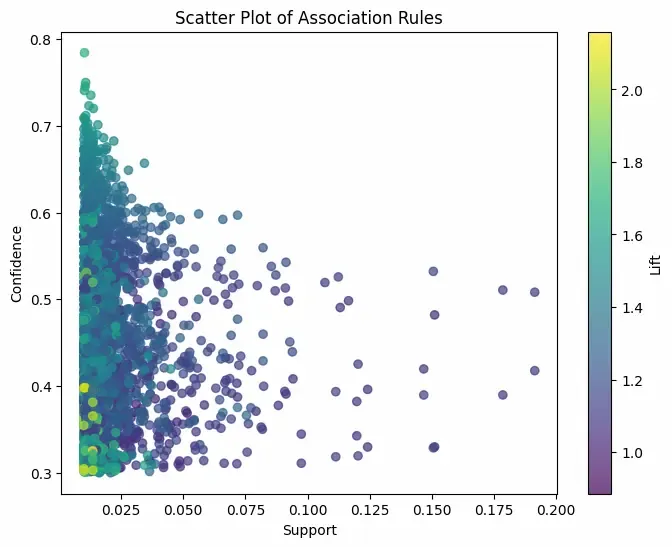
When analyzing this plot, you can see several patterns:

• Rules with high support (far to the right) involve very common items, but their lift may not be exceptional.
• Rules with high confidence (near the top) are very reliable.
• The most "interesting" rules are often those with the highest lift (the brightest colors, in this case yellow/green), as they represent the strongest associations beyond what's expected by chance. A stylist might prioritize these high-lift rules to create surprising yet effective combinations.

Numerical Exercise

Let's apply these concepts. You have a small dataset of 10 recent, successful photoshoot looks. Your task is to evaluate a potential styling rule.

Dataset (10 Looks):

1. {Plunge Bra, Thong, Black}
2. {Balconette Bra, Brief, White}
3. {Plunge Bra, Thong, Red}
4. {Bralette, Thong, Black}
5. {Plunge Bra, Brief, Black}
6. {Balconette Bra, Thong, White}
7. {Plunge Bra, Thong, Black}
8. {Bralette, Brief, Red}
9. {Balconette Bra, Brief, Black}
10. {Plunge Bra, Thong, Red}

Your Task:
For the association rule $\{\text{Plunge Bra}\}\to \{\text{Thong}\}$, calculate the Support, Confidence, and Lift. Based on your results, would you consider this a strong rule for your styling guide?

Take a moment to work through the calculations before revealing the solution.

Solution and Interpretation

Let's break down the calculations.

• Total number of looks (transactions) = 10.
• Number of looks with {Plunge Bra} = 5. (Looks 1, 3, 5, 7, 10)
• Number of looks with {Thong} = 6. (Looks 1, 3, 4, 6, 7, 10)
• Number of looks with both {Plunge Bra, Thong} = 4. (Looks 1, 3, 7, 10)

1. Support: We calculate the support of the combined itemset.

   $$\text{Support}(\{\text{Plunge Bra, Thong}\})=\frac{4}{10}=0.4$$

2. Confidence: We calculate the confidence of the rule $\{\text{Plunge Bra}\}\to \{\text{Thong}\}$.

   $$\text{Confidence}=\frac{\text{Support}(\{\text{Plunge Bra, Thong}\})}{\text{Support}(\{\text{Plunge Bra}\})}=\frac{4/10}{5/10}=\frac{4}{5}=0.8$$

3. Lift: We calculate the lift of the rule.

   $$\text{Lift}=\frac{\text{Confidence}}{\text{Support}(\{\text{Thong}\})}=\frac{0.8}{6/10}=\frac{0.8}{0.6}\approx 1.33$$

Interpretation:

• The Support of 0.4 is quite high, indicating this is a very common pairing in your successful looks.
• The Confidence of 0.8 is also very high. It means that 80% of the time you've used a Plunge Bra, a Thong was the chosen bottom. This is a highly reliable rule.
• The Lift of 1.33 tells us that this pairing occurs 33% more often than we'd expect if the choices were independent. It's a positive association.

Conclusion: Yes, this is a strong and useful rule. The high confidence and support make it a reliable, mainstream choice for your styling guide. The positive lift confirms there is a genuine stylistic synergy between the two pieces.

Conclusion

In this lesson, you've learned how to apply association rule mining to discover meaningful relationships between lingerie pieces in a collection of outfits. You now understand how to move beyond simple frequency counts and evaluate these relationships using the robust statistical metrics of support, confidence, and lift. This provides a data-driven method for one of the most crucial creative tasks: building a cohesive and compelling look.

Key Takeaways:

• Association Rule Mining can be adapted from "market baskets" to "photoshoot outfits" to find pairing rules.
• Support measures the popularity of an itemset.
• Confidence measures the reliability of a rule ($P(Y|X)$).
• Lift measures the "interestingness" of a rule by comparing its probability to what would be expected from random chance, making it the key metric for discovering strong, non-obvious associations.

Preview of the Next Lesson:
We have just explored how to find relationships between items. In our next lesson, we will shift our focus to finding relationships between people (or in your case, models). We will explore Collaborative Filtering, a technique that powers recommendation engines. You'll learn how to predict a model's rating for a new lingerie style by leveraging the ratings of other models with similar tastes, adding another powerful tool for personalized style optimization.