Predicting Lingerie Ratings with User-Based Collaborative Filtering

The Problem of Predicting Preference

At its core, the recommendation problem is about filling in the blanks. Imagine a large table where rows represent your models and columns represent all the lingerie pieces you've ever used. The cells contain the rating each model gave to each piece, but most cells are empty because no model has tried every single item. Our goal is to predict these missing values.

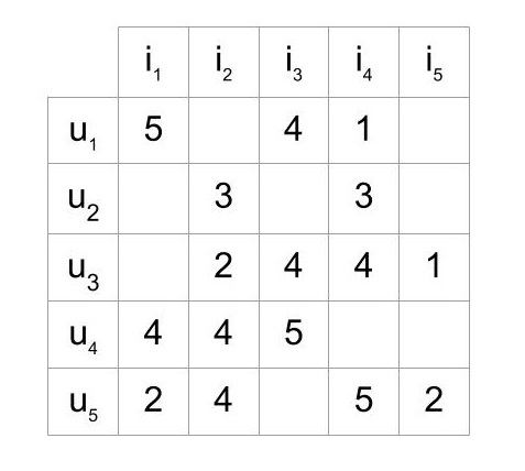
This process of "filling in the matrix" can be approached in several ways. One powerful method is collaborative filtering, which leverages the "wisdom of the crowd."

User-Based vs. Item-Based Filtering

Collaborative filtering primarily splits into two approaches, both starting from the same rating matrix but taking different paths to find a prediction.

1. User-Based Collaborative Filtering (our focus today): The core idea is "If model A and model B have similar tastes, then model A will likely enjoy other lingerie pieces that model B has enjoyed." We find a 'neighborhood' of similar models and use their ratings to predict the target model's rating for a new item.

2. Item-Based Collaborative Filtering: The idea here is "If a model liked a specific lace balconette bra, she will probably also like other similar lace balconette bras." This involves finding similar items and predicting a rating based on how the model rated those similar items.

While both are powerful, we will concentrate on the user-based approach as specified in our learning goal.

Step 1: Finding Models with Similar Tastes

The most critical step in user-based collaborative filtering is to mathematically define and calculate "similar tastes." How can we quantify the similarity between two models, say Alice and Brenda, based on their rating history?

A simple approach might be to look at the movies... I mean, lingerie... they've both rated. However, as your statistical background will tell you, a simple count or basic similarity measure can be misleading. A more robust method is needed that accounts for individual rating behavior. For instance, Alice might be a "tough rater" who rarely gives a score above 4, while Brenda is an "easy rater" who hands out 5s freely.

To handle this, we use Centered Cosine Similarity, which you'll know by another name: the Pearson correlation coefficient.

The process, as explained in the video, is as follows:

1. For each model, calculate her average rating across all the items she has rated.
2. Create a new, "centered" rating matrix by subtracting this average from each of her individual ratings. Now, a positive rating means she liked an item more than her personal average, a negative rating means she liked it less, and a zero represents an average rating.
3. Calculate the cosine similarity between the vectors of two models using this new centered matrix. This value is the Pearson correlation coefficient, $w_{uv}$, between model $u$ and model $v$. It will range from -1 (perfectly opposite tastes) to +1 (identical tastes).

Step 2: Predicting the Rating

Once we have a way to calculate the similarity $w_{uv}$ between our target model $u$ and all other models $v$, we can predict her rating for a new lingerie piece, $i$.

The logic is to find a neighborhood of the k most similar models to $u$ who have already rated item $i$, and then calculate a weighted average of their ratings. The weights are their similarity scores. A model with a similarity of 0.9 to our target model will have her opinion count much more than a model with a similarity of 0.2.

The prediction formula looks like this. Given your operations research background, this formulation of a weighted sum should be quite familiar.

Let's break down that final prediction formula from the paper:

${\hat{v}}_{ui}={\bar{v}}_u+\frac{{\sum }_{v\in N}{w}_{uv}(v_{vi}-{\bar{v}}_v)}{{\sum }_{v\in N}|w_{uv}|}$

Where:

• ${\hat{v}}_{ui}$ is the predicted rating of model $u$ for item $i$.
• ${\bar{v}}_u$ is the average rating of our target model $u$.
• $N$ is the neighborhood of similar models who have rated item $i$.
• $w_{uv}$ is the Pearson correlation (similarity) between models $u$ and $v$.
• $v_{vi}-{\bar{v}}_v$ is the centered rating of neighbor model $v$ for item $i$.

In essence, we are calculating the weighted average of how much the other models deviated from their own average for this item, and then adding that deviation to our target model's average rating. This accounts for the fact that our target model might be a "tough rater" herself.

Numerical Exercise

Let's put this into practice. You are trying to predict how a model, Carla, will rate the 'Satin Chemise'. You have a rating matrix from three other models: Alice, Brenda, and Dana. Ratings are on a 1-5 scale.

Your Task: Predict Carla's rating for the 'Satin Chemise' using user-based collaborative filtering. Use a neighborhood of the two most similar models (k=2).

1. Calculate Mean Ratings: Find the average rating for each model who has rated the 'Satin Chemise' (Alice, Brenda, Dana) and for Carla.
2. Calculate Similarities: Calculate the Pearson correlation between Carla and the other three models. Remember to only use items they have both rated.
   • Carla-Alice: Use 'Plunge Bra' and 'Lace Bodysuit'.
   • Carla-Brenda: Use 'Plunge Bra', 'Lace Bodysuit', and 'Garter Belt'.
   • Carla-Dana: Use 'Plunge Bra' and 'Garter Belt'.
3. Identify the Neighborhood: Select the two models with the highest similarity score to Carla.
4. Predict the Rating: Use the weighted average formula to calculate the final predicted rating for Carla on the 'Satin Chemise'.

Take your time to work through the steps. The solution is below.

Solution

1. Calculate Mean Ratings:

• ${\bar{v}}_{\text{Alice}}=(5+4+4)/3=4.33$
• ${\bar{v}}_{\text{Brenda}}=(2+3+3+2)/4=2.5$
• ${\bar{v}}_{\text{Dana}}=(5+5+4)/3=4.67$
• ${\bar{v}}_{\text{Carla}}=(4+3+5)/3=4.0$

2. Calculate Similarities (Pearson Correlation):
Let's use the standard formula for Pearson's $r$:
$r=\frac{\sum (x_i-\bar{x})(y_i-\bar{y})}{\sqrt{\sum (x_i-\bar{x}{)}^2\sum (y_i-\bar{y}{)}^2}}$

• Similarity(Carla, Alice):

  • Items in common: Plunge Bra, Lace Bodysuit.
  • Carla's ratings: (4, 3). $\bar{x}=3.5$. Centered: (0.5, -0.5).
  • Alice's ratings: (5, 4). $\bar{y}=4.5$. Centered: (0.5, -0.5).
  • Numerator: $(0.5)(0.5)+(-0.5)(-0.5)=0.25+0.25=0.5$
  • Denominator: $\sqrt{(0.5^2+(-0.5{)}^2)}\times \sqrt{(0.5^2+(-0.5{)}^2)}=\sqrt{0.5}\times \sqrt{0.5}=0.5$
  • $w_{\text{Carla,Alice}}=0.5/0.5=1.0$. (Perfect correlation on the items they share).

• Similarity(Carla, Brenda):

  • Items: Plunge Bra, Lace Bodysuit, Garter Belt.
  • Carla's ratings: (4, 3, 5). $\bar{x}=4.0$. Centered: (0, -1, 1).
  • Brenda's ratings: (2, 3, 2). $\bar{y}=2.33$. Centered: (-0.33, 0.67, -0.33).
  • Numerator: $(0)(-0.33)+(-1)(0.67)+(1)(-0.33)=-0.67-0.33=-1.0$
  • Denominator: $\sqrt{0^2+(-1{)}^2+1^2}\times \sqrt{(-0.33{)}^2+0.67^2+(-0.33{)}^2}=\sqrt{2}\times \sqrt{0.11+0.45+0.11}=\sqrt{2}\times \sqrt{0.67}=1.414\times 0.819=1.158$
  • $w_{\text{Carla,Brenda}}=-1.0/1.158=-0.86$

• Similarity(Carla, Dana):

  • Items: Plunge Bra, Garter Belt.
  • Carla's ratings: (4, 5). $\bar{x}=4.5$. Centered: (-0.5, 0.5).
  • Dana's ratings: (5, 4). $\bar{y}=4.5$. Centered: (0.5, -0.5).
  • Numerator: $(-0.5)(0.5)+(0.5)(-0.5)=-0.25-0.25=-0.5$
  • Denominator: $\sqrt{(-0.5{)}^2+0.5^2}\times \sqrt{0.5^2+(-0.5{)}^2}=\sqrt{0.5}\times \sqrt{0.5}=0.5$
  • $w_{\text{Carla,Dana}}=-0.5/0.5=-1.0$

3. Identify the Neighborhood (k=2):
The models who have rated 'Satin Chemise' are Alice, Brenda, and Dana.

• Similarity(Carla, Alice) = 1.0
• Similarity(Carla, Brenda) = -0.86
• Similarity(Carla, Dana) = -1.0

The two most similar models are Alice ($w=1.0$) and Brenda ($w=-0.86$). So, $N=\{\text{Alice, Brenda}\}$. Note: Even though Brenda has a negative correlation, she is 'more similar' than Dana, who has a perfect negative correlation.

4. Predict the Rating:
${\hat{v}}_{\text{Carla,SC}}={\bar{v}}_{\text{Carla}}+\frac{w_{\text{C,A}}(v_{\text{A,SC}}-{\bar{v}}_{\text{A}})+w_{\text{C,B}}(v_{\text{B,SC}}-{\bar{v}}_{\text{B}})}{|w_{\text{C,A}}|+|w_{\text{C,B}}|}$

• ${\bar{v}}_{\text{Carla}}=4.0$
• Alice's rating for SC: $v_{\text{A,SC}}=4$. ${\bar{v}}_{\text{A}}=4.33$. Deviation: $4-4.33=-0.33$.
• Brenda's rating for SC: $v_{\text{B,SC}}=3$. ${\bar{v}}_{\text{B}}=2.5$. Deviation: $3-2.5=0.5$.

${\hat{v}}_{\text{Carla,SC}}=4.0+\frac{(1.0)(-0.33)+(-0.86)(0.5)}{|1.0|+|-0.86|}$
${\hat{v}}_{\text{Carla,SC}}=4.0+\frac{-0.33-0.43}{1.86}=4.0+\frac{-0.76}{1.86}=4.0-0.41=3.59$

Predicted rating: ~3.6. Based on the tastes of similar models, Carla is predicted to rate the 'Satin Chemise' around 3.6 out of 5.

Conclusion

In this lesson, you've learned the mechanics of user-based collaborative filtering, a method to predict a model's preferences for items she hasn't seen. By leveraging your statistical foundation, you can now appreciate the importance of using a robust similarity metric like Pearson correlation and understand how to combine the opinions of a "neighborhood" of similar users into a single, actionable prediction.

Key Takeaways:

• User-based collaborative filtering predicts ratings for a target user by finding a neighborhood of similar users.
• Pearson correlation is an effective similarity metric because it mean-centers each user's ratings, accounting for individual biases.
• A weighted average of the neighbors' centered ratings, adjusted by the target user's own average, provides a robust prediction.
• This technique is powerful but faces challenges, notably the "cold start" problem: it cannot make predictions for new models with no rating history, nor can it recommend new items that no one has rated yet.

Preview of the Next Lesson:
We have now covered methods for discovering item pairings and for predicting individual preferences. This concludes our module on advanced optimization techniques. In our final lesson of this module, we will tackle a different kind of optimization problem directly relevant to the "Fitting Room Experimentation" phase: Optimal Stopping. You will learn a famous rule to decide when to stop scouting for new lingerie options and commit to the best one you have seen so far, maximizing your chances of making the perfect final selection for the photoshoot.