Spearman Correlation for Lingerie Design Analysis

In our last lesson, we explored how Pearson correlation can reveal linear relationships in your data, such as the strong positive link we found between a plunge bra's neckline depth and its appeal score. However, as you know from your statistical background, not all meaningful relationships follow a straight line. What happens when an attribute's appeal increases steadily but not at a constant rate?

This lesson addresses that exact scenario. Our objective is to apply Spearman rank correlation to assess monotonic relationships, which are common in aesthetic judgments. You will learn to use this powerful non-parametric tool to analyze connections between ordinal data, like a model's preference rankings, and specific design attributes of your lingerie pieces. This moves us beyond simple linear trends into a more nuanced understanding of what makes a style successful.

Beyond Linearity: Understanding Monotonic Relationships

Before we dive into the calculation, let's clarify the type of relationship Spearman correlation is designed to detect. While Pearson correlation measures how well data fits a straight line, Spearman correlation measures how well the relationship can be described by a monotonic function.

A monotonic relationship is one where:

As one variable increases, the other variable never decreases (positive monotonic).
As one variable increases, the other variable never increases (negative monotonic).

The key is consistency in direction, not rate. For example, increasing the "delicacy" of lace on a teddy might consistently increase its perceived "romance" score, but the effect might have diminishing returns. The first few details add a lot; subsequent details add less. The relationship is not linear, but it is monotonic.

These plots illustrate the concept. The first two show monotonic relationships (one negative, one positive but non-linear), where the trend is consistent. The third shows a non-monotonic relationship, where the trend reverses. Spearman correlation is designed for the first two cases.

Spearman's $ρ$ : Pearson's Logic on Ranked Data

The elegance of Spearman's rank correlation coefficient, denoted by $ρ$ (rho) or $r_{s}$ , is that it leverages a concept you already know well. It is simply the Pearson correlation coefficient calculated on the ranks of the variables, rather than their raw values.

This video provides an excellent intuitive explanation for why this is so powerful.

Spearman Correlation - Simply Explained

The video "Spearman Correlation - Simply Explained" from the ritvikmath channel clearly explains the limitations of Pearson and the purpose of Spearman.

Watch the entire video. Pay close attention to the basketball and bowling example from the beginning, as it perfectly illustrates a non-linear but perfectly monotonic relationship. The core insight is explained from the moment the video introduces ranks, showing how transforming data into ranks allows us to use the familiar Pearson formula to capture a different kind of association.

By converting data to ranks, we abstract away the specific values and focus only on their relative order. This makes the method robust to outliers and, crucially, allows it to detect monotonic relationships that are not linear.

The following table from the GeeksforGeeks article "Spearman's Rank Correlation" neatly summarizes the key differences from Pearson correlation.

Spearman's Rank Correlation - GeeksforGeeks

This article provides a concise reference for Spearman's \rho. This section offers a clear comparison table.

Review the table under the heading "Difference Between Pearson and Spearman Correlation". The key distinctions are the data type (ordinal or continuous for Spearman), the use of ranks, the lack of a normality assumption, and the type of relationship measured (monotonic vs. linear).

Numerical Exercise: Sheerness vs. Model Preference

Let's apply this to your "Aphrodite" photoshoot project. Imagine you're trying to understand if there's a relationship between the sheerness of a lingerie piece and your model's personal preference. You have data on eight distinct pieces. For each, you have a "Sheerness Score" (a 1-100 scale you've devised based on fabric opacity) and the model's preference ranking for the shoot (1st choice, 2nd choice, etc.).

Here is the data:

Piece ID	Style	Sheerness (x)	Model's Rank (y)
A	Lace Bodysuit	80	2
B	Silk Robe	20	7
C	Mesh Teddy	95	1
D	Cotton Bralette	5	8
E	Satin Chemise	40	6
F	Garter Belt Set	70	4
G	Open-Cup Bra	80	3
H	Strappy Panty	85	5

Your task is to calculate Spearman's rank correlation, $ρ$ , to assess the monotonic relationship between sheerness and model preference.

We will use the formula for Spearman's rho when there are no or few ties:

ρ = 1 - \frac{6 \sum d ^{2}}{n ( n ^{2} - 1 )}

where $d$ is the difference between the ranks of each pair of values, and $n$ is the number of pairs.

The following resource walks through the exact steps for this calculation.

Spearman's Rank Correlation - GeeksforGeeks

This section from GeeksforGeeks provides a clear, step-by-step guide to the manual calculation.

Follow the logic outlined in the section "Calculating Spearman’s Rank Correlation". You will need to perform these steps on our lingerie dataset. Pay close attention to how they handle tied ranks, as this is relevant to our data.

Your Task:

Create a table. Your columns should be: Piece ID, Sheerness (x), Rank of x, Model's Rank (y), Rank difference (d), and $d^{2}$ .
Rank the 'Sheerness' variable. Assign rank 1 to the lowest score, 2 to the next lowest, and so on. Remember to handle the tie for the Sheerness score of 80 by assigning the average of the ranks they would have occupied.
The 'Model's Rank' is already ranked, so you can use those values directly.
Calculate $d$ and $d^{2}$ .
Sum the $d^{2}$ column to get $\sum d^{2}$ .
Substitute the values into the formula to find $ρ$ .

Click to see the detailed solution.

Step 1 & 2: Rank the 'Sheerness' data and create the table.

First, let's order the pieces by Sheerness to make ranking easier:

D (5) -> Rank 1
B (20) -> Rank 2
E (40) -> Rank 3
F (70) -> Rank 4
A (80) & G (80) -> These would occupy ranks 5 and 6. The average rank is (5+6)/2 = 5.5.
H (85) -> Rank 7
C (95) -> Rank 8

Now we can build the full table.

Piece ID	Sheerness (x)	Rank of x	Model's Rank (y)	d = Rank(x) - Rank(y)	$d^{2}$
A	80	5.5	2	3.5	12.25
B	20	2	7	-5.0	25.00
C	95	8	1	7.0	49.00
D	5	1	8	-7.0	49.00
E	40	3	6	-3.0	9.00
F	70	4	4	0.0	0.00
G	80	5.5	3	2.5	6.25
H	85	7	5	2.0	4.00
Sum					154.5

Step 3, 4, & 5: Calculate sums.

$n = 8$
$\sum d^{2} = 154.5$

Step 6: Plug the values into the formula.

ρ = 1 - \frac{6 \times 154.5}{8 ( 8 ^{2} - 1 )}

ρ = 1 - \frac{927}{8 ( 63 )}

ρ = 1 - \frac{927}{504}

ρ = 1 - 1.839

ρ \approx - 0.839

The Spearman rank correlation coefficient is approximately $ρ = - 0.84$ .

Interpreting the Result

Our calculated $ρ \approx - 0.84$ indicates a strong negative monotonic relationship.

Direction: The value is negative. This means as one variable's rank increases, the other's tends to decrease. In our context, as the Sheerness score rank increases (i.e., the garment becomes sheerer), the model's preference rank tends to decrease (i.e., she prefers it more, since rank 1 is the top preference). Therefore, the model consistently prefers sheerer garments.
Strength: A value of -0.84 is close to -1, indicating a strong relationship. The model's preference for sheerness is not random; it's a very consistent trend.

This visual comparison demonstrates how Spearman correlation can give a more intuitive result for a monotonic, non-linear trend compared to Pearson.

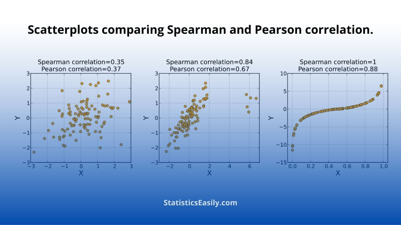
Notice the plot on the far right. The relationship is perfectly monotonic—as X increases, Y always increases. Spearman correlation is a perfect 1. However, because it's not a straight line, Pearson correlation is only 0.88. This highlights Spearman's strength in capturing consistent trends regardless of linearity.

Finally, it is worth noting that Spearman correlation is widely used in academic research on fashion and aesthetics to assess agreement and ranking consistency, reinforcing its utility for your project.

A Dataset for Aesthetics-Aligned Clothing Outfit Recommendation

This paper from a top AI conference discusses creating a dataset for clothing recommendations. The authors use statistical methods to validate their data.

First, read the brief paragraph under the heading "Validation Metrics," which explicitly defines Spearman rank correlation as a key metric "to measure ranking consistency with robustness to outliers." Then, skim the paragraph under "Domain-Specific Validation," where the authors report both Pearson and Spearman coefficients to measure the agreement between human fashion experts and an AI model. This shows how both measures are used together in practice.

Conclusion

In this lesson, you've expanded your toolkit for analyzing relationships by mastering Spearman rank correlation. You can now confidently assess monotonic trends, which are often more representative of aesthetic preferences than purely linear ones.

Key Takeaways:

Spearman's $ρ$ measures the strength and direction of a monotonic relationship.
It operates on the ranks of the data, making it suitable for ordinal variables (like preference rankings) and robust to outliers.
The calculation involves ranking each variable, finding the differences, and applying the Spearman formula. A value near +1 or -1 indicates a strong monotonic association.

You've now compared two variables with Pearson correlation and two sets of ranks with Spearman correlation. But what if you need to assess the agreement among multiple people? For instance, what if your model, photographer, and stylist all rank the same set of lingerie? Is there consensus? Our next lesson will introduce Kendall's W, a statistic designed specifically to measure this kind of inter-rater reliability.

Recommended resources

Beyond Linearity: Understanding Monotonic Relationships

Spearman's ρ: Pearson's Logic on Ranked Data

Numerical Exercise: Sheerness vs. Model Preference

Interpreting the Result

Conclusion

Spearman's $ρ$ : Pearson's Logic on Ranked Data