Random Walks and Diffusion: A Dimensional Analysis Approach

Introduction

In our last lesson, we saw how dimensional analysis can be a powerful tool for deducing the scaling behavior of static physical quantities, such as the Fermi energy in an electron gas or the Debye temperature in a solid. By identifying the handful of physical parameters that govern a system, we were able to predict its fundamental energy scales.

This lesson concludes our first module by extending this heuristic approach from static properties to dynamic processes. We will focus on one of the most fundamental models in all of statistical physics: the random walk. Your objective is to apply dimensional analysis and scaling arguments to derive the characteristic scaling behavior of a random walk and, crucially, to understand its deep connection to the macroscopic process of diffusion. This concept is foundational in condensed matter physics, describing phenomena from charge carrier motion in semiconductors to the dynamics of polymers, and it serves as a perfect prototype for the scaling ideas central to the renormalization group.

The Scaling of a Random Walk

Imagine a particle starting at an origin and taking a series of discrete steps. At each time interval $τ$ , it moves a fixed distance $l_{0}$ , but the direction is chosen randomly. After many steps, where does the particle end up?

By symmetry, the average position of the particle will remain at the origin, $⟨ x ⟩ = 0$ . A more informative measure is the root-mean-square (RMS) displacement from the origin, $x_{r m s} = ⟨ x^{2} ⟩$ . How does this characteristic distance scale with the number of steps, $N$ ?

The top plot shows three distinct trajectories of a one-dimensional random walk. Notice how each path is erratic and unpredictable. The bottom plot shows the mean squared displacement, $\langle x^2 \rangle$, averaged over many such walks, as a function of the number of steps $N$. The clear linear trend suggests a simple power-law relationship.

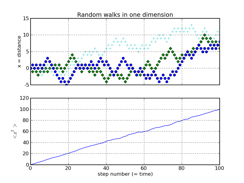
A direct calculation can provide the answer.

The Random Walk

The video "The Random Walk" from the Think Like a Physicist channel provides a clear derivation of the standard deviation of the particle's position.

Please watch the final segment of the video that begins with the calculation of the standard deviation. Focus on the steps from calculating the standard deviation of the number of rightward steps, M, to finding the standard deviation of the final position, X. The conclusion of this calculation is the central scaling law we are seeking.

As the video demonstrates, the standard deviation of the position after $N$ steps is $N$ (assuming a step length of 1). In general, for a step length $l_{0}$ , the mean-squared displacement is:

⟨ x^{2} ⟩ = N l_{0}^{2}

This implies that the characteristic distance from the origin grows as the square root of the number of steps:

x_{r m s} = ⟨ x^{2} ⟩ = l_{0} N

This $x_{r m s} \propto N^{1/2}$ scaling is a hallmark of diffusive processes. It's a non-trivial result; a naive guess might have suggested the distance scales linearly with $N$ , which would only be true if all the steps were in the same direction. The random nature of the walk fundamentally changes the scaling behavior.

A Scaling Argument: The Random Walk as a Fractal

While the probabilistic derivation is exact, we can also deduce the scaling exponent $ν = 1/2$ using a more physical, RG-style scaling argument. This type of reasoning is central to modern theoretical physics and aligns with your interest in the renormalization group. The core idea is self-similarity: a long random walk looks statistically similar to a shorter random walk with larger steps.

[PDF] renormalization and scaling in applied mathematics gunduz caginalp

Gunduz Caginalp's tutorial notes provide a very clear illustration of this scaling argument.

Please read the section titled "RANDOM WALK - Basic". Pay close attention to the logic in the subsection "An Alternative Look". The argument begins by positing a general scaling form, R(M;s), and then enforces consistency between a microscopic description and a coarse-grained one to find the exponent \nu.

Let's formalize this powerful argument.

Assume a scaling form. Based on dimensional analysis, the RMS displacement $R$ after $M$ steps of size $s$ must be proportional to $s$ . The dependence on the dimensionless number of steps $M$ is likely a power law. So we posit:
$R (M; s) \sim s M^{ν}$
Our goal is to determine the exponent $ν$ .
Coarse-grain. Imagine grouping the $M$ microscopic steps into $M / n$ blocks, where each block contains $n$ steps.
Find the new effective step size. From our scaling law, the RMS size of one of these new "macro-steps" is $s^{'} = R (n; s) \sim s n^{ν}$ .
Enforce self-similarity. The total RMS displacement must be the same whether we view it as $M$ micro-steps of size $s$ or as $M / n$ macro-steps of size $s^{'}$ . We equate the two descriptions:
$R (M; s) = R (M / n; s^{'})$
Substituting our scaling forms:
$s M^{ν} \sim s^{'} (M / n)^{ν} = (s n^{ν}) (M / n)^{ν} = s n^{ν} M^{ν} n^{- ν} = s M^{ν}$
Whoops. This looks like a tautology. Let's re-examine the argument in the resource. The key is to use the known scaling for the coarse-grained step. We know from the direct calculation that a walk of $n$ steps has an RMS size of $n s$ . Let's use that.

Let's try again, following Caginalp's and McGreevy's logic more closely.

We still assume $R (M; s) \sim s M^{ν}$ .
We coarse-grain the $M$ -step walk into $M / n$ steps.
The new effective step size $s^{'}$ is the RMS size of an $n$ -step sub-walk. From the direct calculation, we know $s^{'} = n s$ .
The total RMS distance, viewed as a walk of $M / n$ steps of size $s^{'}$ , must be $R (M / n; s^{'}) = s^{'} (M / n)^{1/2}$ , assuming the $N$ law holds for any walk.
But from our initial scaling hypothesis for the full walk, this distance must also be $s M^{ν}$ . Wait, this is also not the argument.

Let's be very precise. The argument is about finding $ν$ without prior knowledge.

Posit $R (M; s) \sim s M^{ν}$ .
The RMS distance for a walk of $M / n$ coarse-grained steps of size $s^{'}$ is $R (M / n; s^{'}) \sim s^{'} (M / n)^{ν}$ .
The coarse-grained step size itself, being a walk of $n$ steps, has an RMS size of $s^{'} \sim s n^{ν}$ .
Substitute (3) into (2): $R \sim (s n^{ν}) (M / n)^{ν} = s n^{ν} M^{ν} n^{- ν} = s M^{ν}$ . This is still a tautology.

Let's follow the McGreevy resource (LINK) carefully. The logic is subtle.

σ M^{ν} = σ^{'} (M^{'})^{ν}

Here, $M^{'} = M / n$ . The crucial insight is that $σ^{'}$ is the RMS size of an $n$ -step walk, which we can calculate directly: $σ^{'2} = n σ^{2} ⟹ σ^{'} = n σ$ . It is not $σ^{'} = σ n^{ν}$ . The argument uses a known result for the sub-problem to constrain the larger problem.

σ M^{ν} = (n σ) (M / n)^{ν} = σ n^{1/2} M^{ν} n^{- ν} = σ M^{ν} n^{1/2 - ν}

For this equation to hold true for any choice of coarse-graining factor $n$ , the exponent of $n$ must be zero.

1/2 - ν = 0 ⟹ ν = 1/2

This is a beautiful and profound argument. It shows that the $N$ scaling is a necessary consequence of the statistical self-similarity of the walk. All microscopic models that coarse-grain in this way (like a random walk with steps drawn from a Gaussian distribution, as shown in the resources) flow to the same large-scale behavior. This is the essence of universality, a concept you will encounter repeatedly in your study of condensed matter and RG.

The Connection to Diffusion

The scaling law $x_{r m s} \propto t$ is not just a feature of a discrete lattice model; it is the signature of the physical process of diffusion. Diffusion is described by the partial differential equation:

\frac{\partial C ( x , t )}{\partial t} = D \frac{\partial ^{2} C ( x , t )}{\partial x ^{2}}

where $C (x, t)$ is the concentration of a substance (or a probability density) and $D$ is the diffusion coefficient.

Let's apply dimensional analysis to the diffusion equation itself.

The Diffusion Equation Part 2: Dimensional Analysis and Self-Similarity

The video "The Diffusion Equation Part 2" provides a clear walkthrough of this dimensional analysis.

Please watch the segment from the start of the dimensional analysis. The goal is to find the dimensions of the diffusion coefficient D (labeled 'a' in the video) and then use that to construct a characteristic length scale from D and time t.

As the video shows, the dimensions of the diffusion coefficient are $[D] = L^{2} T^{- 1}$ . To find the characteristic distance $x$ that a particle diffuses in time $t$ , we must combine $D$ and $t$ to form a quantity with dimensions of length.
Assuming a power-law relationship $x \propto D^{a} t^{b}$ :

L^{1} T^{0} = [L^{2} T^{- 1}]^{a} [T]^{b} = L^{2 a} T^{b - a}

Equating the exponents for $L$ and $T$ gives a system of two equations:

$1 = 2 a$
$0 = b - a$

Solving this gives $a = 1/2$ and $b = 1/2$ . Therefore, the characteristic length scale for diffusion is:

x \propto D t

This is exactly the same scaling with time that we found for the random walk!

This plot shows the solution to the diffusion equation, $W(x,t)$, starting from a particle localized at $x=0$ at $t=0$. At later times, the probability distribution spreads out as a Gaussian. The width of this Gaussian, which corresponds to the RMS displacement, grows with time, visually demonstrating the $x \propto \sqrt{t}$ scaling.

The identical scaling is no coincidence. The diffusion equation is the macroscopic, continuum limit of the microscopic random walk. We can make the connection explicit by relating the microscopic parameters of the walk ( $l_{0}$ , $τ$ ) to the macroscopic diffusion coefficient $D$ .

For the random walk, we found $⟨ x^{2} ⟩ = N l_{0}^{2} = (t / τ) l_{0}^{2}$ .
A full solution of the 1D diffusion equation for a particle starting at the origin shows that $⟨ x^{2} ⟩ = 2 D t$ .

Equating these two expressions for the mean-squared displacement gives:

2 D t = \frac{t}{τ} l_{0}^{2} ⟹ D = \frac{l _{0}^{2}}{2 τ}

This remarkable formula shows how a macroscopic transport coefficient, $D$ , which can be measured in a lab, is determined by the microscopic details of the random motion—the square of the step length divided by twice the time per step. This is a classic example of how statistical mechanics bridges the microscopic and macroscopic worlds.

Conclusion

In this final lesson of the module, you've used dimensional analysis and scaling arguments to dissect the dynamics of a random walk, a cornerstone model in physics. You have seen that its characteristic scaling behavior is intimately linked to the macroscopic phenomenon of diffusion.

Key Takeaways:

Diffusive Scaling: The root-mean-square displacement of an unbiased random walk scales with the square root of the number of steps or time, $x_{r m s} \propto N \propto t$ . This is fundamentally different from ballistic motion where distance is linear in time.
Scaling from Self-Similarity: The $ν = 1/2$ exponent can be derived elegantly through an RG-style argument that relies on the statistical self-similarity of the walk across different length scales.
Diffusion as a Continuum Limit: The diffusion equation is the macroscopic description of an underlying microscopic random walk. Its characteristic length scale, $x \propto D t$ , exhibits the same scaling.
Bridging Scales: The diffusion coefficient $D$ provides a direct link between the microscopic parameters of the walk (step size $l_{0}$ , step time $τ$ ) and the observable macroscopic behavior.

You have now completed the first module on Dimensional Analysis and Natural Scales. You have developed a powerful set of heuristics for identifying characteristic scales, simplifying problems, deriving scaling laws, and estimating physical quantities.

In our next module, "Order-of-Magnitude Estimation," we will build upon these skills. While dimensional analysis gives us the correct scaling, order-of-magnitude estimation, or Fermi problems, will equip you with the tools to get the dimensionless prefactors right to within a factor of a few, allowing for rapid, back-of-the-envelope calculations that are indispensable in a physicist's toolkit.

Recommended resources

Introduction

The Scaling of a Random Walk

A Scaling Argument: The Random Walk as a Fractal

The Connection to Diffusion

Conclusion