Dimensional Analysis in Quantum and Statistical Physics

The Power of Dimensional Arguments in Quantum and Statistical Physics

Before tackling specific case studies, let's establish our core heuristic. For many problems in quantum and statistical mechanics, the essential physics is captured by a handful of fundamental constants and system parameters. Once these are identified, dimensional analysis can often uniquely determine the functional form of the quantity we wish to estimate, up to a dimensionless constant of order one.

A classic example from statistical physics is the Stefan-Boltzmann law for blackbody radiation. The intensity of radiation, $I$, must depend on the fundamental constants governing thermodynamics ($k_B$), relativity ($c$), and quantum mechanics ($\hslash$), as well as the temperature $T$.

The analysis shows that the only combination of these parameters that yields the dimensions of intensity ($\text{Energy}/(\text{Area}\cdot \text{Time})$ or $M{T}^{-3}$) is $I\propto (k_{B}T{)}^4/({\hslash }^3{c}^2)$. This immediately tells us that the intensity scales as the fourth power of temperature, $I\propto T^4$, a profound result derived purely from dimensional consistency. The dimensionless prefactor (${\pi }^2/60$) requires a full quantum statistical calculation, but the essential physics is captured by the scaling.

Let's apply this same thinking to a simple quantum system. Consider the quantum harmonic oscillator, with a particle of mass $m$ oscillating at a natural frequency $\omega$. The ground-state energy, $E_0$, can only depend on $m$, $\omega$, and $\hslash$.

• $[E_0]=M{L}^2{T}^{-2}$
• $[\hslash ]=M{L}^2{T}^{-1}$
• $[\omega ]=T^{-1}$
• $[m]=M$

Notice that mass $m$ cannot be part of the final expression. If we include $m$, we can't cancel the dimension of mass without also changing the power of $\hslash$, which would then leave an uncancelled dimension of length. The only way to construct a quantity with dimensions of energy is by combining $\hslash$ and $\omega$. This leads directly to:

This simple dimensional argument correctly predicts that the energy levels of the quantum harmonic oscillator are spaced by $\hslash \omega$. The exact result, $E_0=\frac{1}{2}\hslash \omega$, includes a dimensionless prefactor of $1/2$, but our heuristic has already revealed the fundamental energy scale.

Case Study 1: The Fermi Energy

Now let's turn to a cornerstone of your condensed matter studies: the degenerate Fermi gas. At absolute zero, a system of $N$ non-interacting fermions (like electrons) in a volume $V$ will occupy the lowest $N$ available single-particle energy states, up to a maximum energy known as the Fermi energy, $E_F$. How does this energy scale depend on the properties of the system?

The relevant physical parameters are:

• The particle number density, $n=N/V$, which has dimensions $[n]=L^{-3}$.
• The mass of a fermion, $m$, with $[m]=M$.
• Planck's constant, $\hslash$, since this is a quantum system, with $[\hslash ]=M{L}^2{T}^{-1}$.

Our goal is to combine $n$, $m$, and $\hslash$ to produce a quantity with the dimensions of energy, $M{L}^2{T}^{-2}$. Let's assume a general form $E_F\propto {\hslash }^a{n}^b{m}^c$ and solve for the exponents by matching the dimensions on both sides.

1. Mass (M): The energy $E_F$ has one power of mass. On the right, mass appears in $\hslash$ and $m$. So, $1=a+c$.
2. Time (T): Energy has $T^{-2}$. On the right, only $\hslash$ has dimensions of time. So, $-2=-a$, which gives $a=2$.
3. Substituting back into the mass equation: $1=2+c$, which gives $c=-1$.
4. Length (L): Energy has $L^2$. On the right, $\hslash$ and $n$ have dimensions of length. So, $2=2a-3b$. Substituting $a=2$, we get $2=4-3b$, which yields $b=2/3$.

Putting it all together, we find the scaling relationship:

This powerful result, derived in minutes, tells us how the characteristic energy of a Fermi gas depends on its density and the particle mass. To see how this scaling emerges from a full calculation and to find the missing dimensionless prefactor, we can turn to a more formal derivation.

As you can see from Tong's notes, the full calculation yields:

where $g_s$ is the spin degeneracy factor (e.g., $g_s=2$ for electrons). Our dimensional analysis perfectly captured the dependence on $\hslash$, $m$, and $n$. The formal derivation, which involves integrating the density of states in momentum space, yields the dimensionless prefactor $(3{\pi }^2{)}^{2/3}$ for spin-1/2 particles.

Case Study 2: The Debye Temperature

Our next example comes from the physics of solids. The Debye model provides a description of the heat capacity of a crystal by treating the collective atomic vibrations as quantized sound waves, or phonons. A key concept in this model is that there must be a maximum phonon frequency, ${\omega }_D$, because a wave's wavelength cannot be shorter than the spacing between atoms. This maximum frequency defines a characteristic temperature scale for the solid, the Debye temperature, $T_D$, given by $k_B{T}_D=\hslash {\omega }_D$.

Let's estimate this maximum frequency, ${\omega }_D$, using dimensional analysis. What are the key physical parameters?

• The number density of atoms, $n=N/V$, with $[n]=L^{-3}$. This sets the scale for the interatomic spacing, $d\sim n^{-1/3}$.
• The speed of sound in the solid, $c_s$, with $[c_s]=L{T}^{-1}$.

We want to construct a frequency ($T^{-1}$) from $n$ and $c_s$.
Let ${\omega }_D\propto n^a{c}_s^b$.

1. Time (T): $-1=-b$, so $b=1$.
2. Length (L): $0=-3a+b$. Substituting $b=1$, we get $3a=1$, so $a=1/3$.

This gives us the scaling:

This result has a clear physical interpretation. Since $n^{1/3}$ is proportional to the inverse of the interatomic distance, $1/d$, our estimate is simply ${\omega }_D\sim c_s/d$. This is precisely the frequency of a sound wave whose wavelength is on the order of the minimum possible wavelength in the crystal lattice. The Debye temperature therefore scales as:

Once again, a more rigorous argument is needed to find the numerical prefactor. The clever argument made by Debye, which you will now read, equates the total number of vibrational modes in the crystal to the number of degrees of freedom of the atoms.

The Debye argument gives ${\omega }_D=(6{\pi }^{2}n{)}^{1/3}{c}_s$, which again confirms the scaling we found with dimensional analysis while providing the prefactor $(6{\pi }^2{)}^{1/3}$. This factor arises from integrating the density of states over a sphere in momentum space.

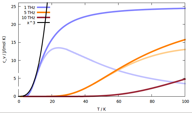
The Debye temperature $T_D$ marks the crossover between two different physical regimes.

• At low temperatures ($T\ll T_D$), only low-frequency, long-wavelength phonons are excited, and the heat capacity is found to be $C_V\propto T^3$.
• At high temperatures ($T\gg T_D$), all $3N$ vibrational modes are excited, and the heat capacity approaches the classical Dulong-Petit value, $C_V=3N{k}_B$.

The heuristic estimation of $T_D$ provides the crucial energy scale that separates these two distinct behaviors.

Conclusion

In this lesson, you've applied the heuristic tools of dimensional analysis and scaling arguments to make concrete estimates for key quantities in quantum and statistical systems. By identifying the essential physical parameters of a problem, we were able to derive the correct functional dependencies for the ground-state energy of an oscillator, the Fermi energy of an electron gas, and the Debye temperature of a solid.

Key Takeaways:

• Dimensional analysis is a predictive tool: It can be used to derive the scaling behavior of physical quantities by combining the relevant parameters and fundamental constants.
• Identify the essential physics: The first step is to determine the minimal set of parameters that govern the phenomenon of interest ($m,\omega ,\hslash$ for the oscillator; $n,m,\hslash$ for the Fermi gas; $n,c_s,\hslash ,k_B$ for the Debye model).
• Scaling reveals behavior: The derived scaling laws—$E_F\propto n^{2/3}$, $T_D\propto n^{1/3}$—provide deep physical insight into how these systems respond to changes in their environment, even before a full calculation is performed.
• Heuristics guide formal calculation: These estimates tell you what to expect from a more rigorous derivation and serve as a crucial sanity check on your results. The full calculations, as seen in the examples from Tong's notes, are often concerned with finding the dimensionless prefactors that our scaling arguments miss.

In the final lesson of this module, we will extend these ideas from static quantities to dynamic processes. You will apply dimensional analysis to derive the scaling behavior of a random walk and see how it provides a fundamental model for the process of diffusion.