Slutsky Equation: Decomposing Price Changes

1. The Intuition: Substitution vs. Income Effects

When the price of a good—say, good 1—falls, two things happen simultaneously:

1. It becomes relatively cheaper: Compared to good 2, good 1 is now a better deal. A rational consumer will tend to substitute away from the more expensive good and towards the cheaper one. This is the substitution effect. It captures the change in consumption due to the change in relative prices alone, as if the consumer's overall well-being (utility) were held constant.
2. Your purchasing power increases: With the same nominal income, you can now afford more than you could before. This is equivalent to an increase in your real income. This change in purchasing power also affects your consumption choices. This is the income effect. It captures the change in consumption due to the change in real income, holding the new relative prices constant.

The total change in demand we observe is the sum of these two effects. Let's visualize this.

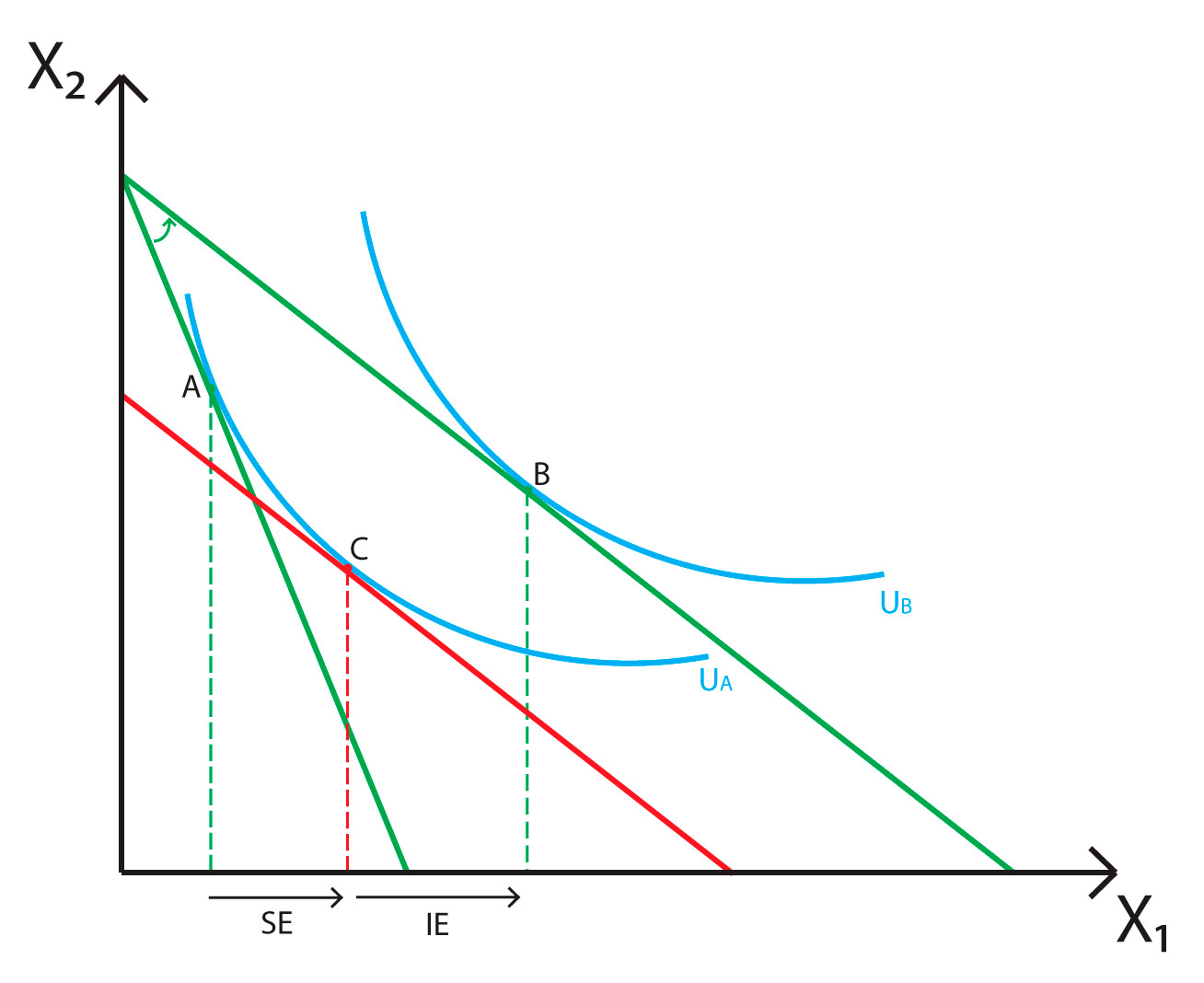
To isolate the substitution effect, we imagine a hypothetical scenario. After the price of good 1 falls, we "compensate" the consumer by taking away just enough income to bring them back to their original indifference curve, $U_A$. The new budget line (dashed green line) has the new price ratio but is tangent to the old indifference curve. The move from A to C is the pure substitution effect. The remaining change, from C to B, is then due purely to the "income" you were given back.

2. The Formal Derivation of the Slutsky Equation

Now, let's translate this intuition into a precise mathematical statement. Your background in physics will make this derivation feel natural, as it's a straightforward application of multivariable calculus.

The starting point is the identity we established in the previous lesson, which connects Hicksian and Marshallian demand:
$h_i(\mathbf{p},u)=x_i(\mathbf{p},e(\mathbf{p},u))$
This equation states that the compensated demand for a good to achieve utility $u$ is identical to the uncompensated demand for that good if the consumer's income is exactly the minimum expenditure, $e(\mathbf{p},u)$, required to reach that utility level.

The following video provides a concise and rigorous derivation of the Slutsky equation by differentiating this identity.

Let's summarize the key steps from the video. We start with the identity and differentiate both sides with respect to the price of another good, $p_j$:

1. Differentiate the identity:
   $\frac{\partial h_i(\mathbf{p},u)}{\partial p_j}=\frac{\partial }{\partial p_j}\left[x_i(\mathbf{p},e(\mathbf{p},u))\right]$
2. Apply the Chain Rule to the right-hand side, since $x_i$ is a function of $p_j$ directly and indirectly through the expenditure function $e$:
   $\frac{\partial h_i}{\partial p_j}=\frac{\partial x_i}{\partial p_j}+\frac{\partial x_i}{\partial e}\frac{\partial e}{\partial p_j}$
3. Apply Shephard's Lemma: We know from our work on expenditure functions that $\frac{\partial e(\mathbf{p},u)}{\partial p_j}=h_j(\mathbf{p},u)$. At the point of optimization, where income $w=e(\mathbf{p},u)$, we also have $h_j(\mathbf{p},u)=x_j(\mathbf{p},w)$. So, $\frac{\partial e}{\partial p_j}=x_j$.
4. Substitute and Rearrange: We also note that a change in expenditure is equivalent to a change in income ($w$), so we can write $\frac{\partial x_i}{\partial e}$ as $\frac{\partial x_i}{\partial w}$. Substituting these back in gives:
   $\frac{\partial h_i}{\partial p_j}=\frac{\partial x_i}{\partial p_j}+\frac{\partial x_i}{\partial w}{x}_j$
   Rearranging to solve for the change in Marshallian demand (the total effect) gives us the Slutsky Equation:
   $\underset{\text{Total Effect}}{\underbrace{\frac{\partial x_i(\mathbf{p},w)}{\partial p_j}}}=\underset{\text{Substitution Effect}}{\underbrace{\frac{\partial h_i(\mathbf{p},u)}{\partial p_j}}}\underset{\text{Income Effect}}{\underbrace{-x_j(\mathbf{p},w)\frac{\partial x_i(\mathbf{p},w)}{\partial w}}}$

This equation is a cornerstone of microeconomic theory. It beautifully decomposes the total change in demand for good $i$ from a price change in good $j$ into its two constituent parts.

3. Interpreting the Effects and Classifying Goods

The Slutsky equation allows us to classify goods based on the signs of the substitution and income effects. Let's focus on the own-price effect ($i=j$).

$\frac{\partial x_i}{\partial p_i}=\frac{\partial h_i}{\partial p_i}-x_i\frac{\partial x_i}{\partial w}$

• Substitution Effect ($\frac{\partial h_i}{\partial p_i}$): This term is always non-positive ($\le 0$). This is known as the Law of Compensated Demand. When a good's price increases, you will never consume more of it if you are compensated to stay on the same indifference curve. Intuitively, you always substitute away from something that has become relatively more expensive.

• Income Effect ($-x_i\frac{\partial x_i}{\partial w}$): The sign of this term depends entirely on how demand for good $i$ changes with income, $\frac{\partial x_i}{\partial w}$.

  • Normal Good: If good $i$ is normal, demand increases with income ($\frac{\partial x_i}{\partial w}>0$). This makes the entire income effect term negative. For a price increase, the income effect reinforces the substitution effect, leading to a definite decrease in demand.
  • Inferior Good: If good $i$ is inferior, demand decreases as income rises ($\frac{\partial x_i}{\partial w}<0$). The income effect term becomes positive. This means the income effect works in the opposite direction to the substitution effect. When the price of an inferior good rises, you feel poorer, so you buy more of it, partially offsetting the fact that you want to substitute away from it.

• Total Effect ($\frac{\partial x_i}{\partial p_i}$):

  • For a normal good, the total effect is unambiguously negative. Demand curves for normal goods always slope downwards.
  • For an inferior good, the total effect is ambiguous. Usually, the negative substitution effect is stronger than the positive income effect, so the demand curve still slopes down.
  • A Giffen good is a special type of inferior good where the positive income effect is so large that it overwhelms the negative substitution effect, causing the total effect to be positive ($\frac{\partial x_i}{\partial p_i}>0$). This means a price increase leads to an increase in quantity demanded—an upward-sloping demand curve. Giffen goods are a theoretical curiosity and extremely rare in practice.

For a rigorous discussion and formal definitions, the following reading is helpful.

4. A Worked Example

Let's ground this theory with a concrete calculation. We'll use the familiar Cobb-Douglas utility function and verify the Slutsky equation holds.

The video demonstrates how to:

1. Derive the ordinary (Marshallian) demand for good X: $x(p_x,p_y,m)$.
2. Calculate the Total Effect by taking the partial derivative: $\frac{\partial x}{\partial p_x}$.
3. Derive the compensated (Hicksian) demand for good X: $h(p_x,p_y,\bar{u})$.
4. Calculate the Substitution Effect by taking the partial derivative: $\frac{\partial h}{\partial p_x}$.
5. Calculate the Income Effect using the formula: $-x\frac{\partial x}{\partial m}$.
6. Verify that Total Effect = Substitution Effect + Income Effect.

This exercise confirms that the abstract equation holds true and gives you a practical feel for how the different components are calculated from the underlying demand functions.

Conclusion

Today, we've unpacked one of the most elegant and powerful results in consumer theory. By linking Marshallian and Hicksian demand, the Slutsky equation provides deep insight into why consumers respond to price changes the way they do.

Key Takeaways:

• The total effect of a price change on quantity demanded can be decomposed into a substitution effect and an income effect.
• The substitution effect captures the response to a change in relative prices, holding utility constant. It is always non-positive for an own-price change.
• The income effect captures the response to a change in purchasing power. Its sign depends on whether the good is normal or inferior.
• The Slutsky equation provides the exact mathematical relationship:
  $\frac{\partial x_i}{\partial p_j}=\frac{\partial h_i}{\partial p_j}-x_j\frac{\partial x_i}{\partial w}$
• This decomposition allows us to classify goods and understand phenomena like Giffen goods, where a strong income effect can overwhelm the substitution effect.

Preview for the Next Lesson:
The Slutsky equation is the central tool for comparative statics—the analysis of how equilibrium quantities (like demand) change when parameters (like prices or income) change. In our next lesson, we will use this framework to more formally analyze how demand curves shift and change shape in response to economic forces, building directly on the decomposition we learned today.