Demand Shifts: Price and Income Effects

1. What is Comparative Statics? The Big Picture

At its core, economic modeling is about building a simplified representation of the world and then running "thought experiments." Comparative statics is the methodology for these experiments. We start with a system in equilibrium, change one parameter, and compare the new equilibrium to the old one.

For the consumer's problem, the equilibrium is the optimal consumption bundle $x^{\ast }(\mathbf{p},w)$. The parameters are prices $\mathbf{p}$ and income $w$. Our "thought experiments" will involve asking questions like:

• How does the optimal bundle change if income increases?
• How does the quantity demanded of good 1 change if its own price rises?
• How does the quantity demanded of good 1 change if the price of good 2 rises?

Mathematically, this amounts to calculating and interpreting the partial derivatives of the Marshallian demand functions. Graphically, it involves tracing how the optimal bundle moves and using that path to derive fundamental relationships like demand curves and Engel curves.

Let's begin by building the graphical intuition for this process.

This video provides the visual foundation. The Price Offer Curve and Income Offer Curve show the path of the optimal bundle in the $(x_1,x_2)$ space as a parameter changes. The Demand Curve and Engel Curve then isolate one good and plot its optimal quantity against the changing parameter. Now, let's formalize these relationships with calculus.

2. Analyzing the Effects of Parameter Changes

A. Income Changes and the Engel Curve

When a consumer's income $w$ changes, the budget constraint shifts in or out in a parallel fashion. The response of demand is captured by the partial derivative with respect to income, $\frac{\partial x_i}{\partial w}$.

• A good is defined as normal if consumption increases as income increases: $\frac{\partial x_i}{\partial w}>0$.
• A good is defined as inferior if consumption decreases as income increases: $\frac{\partial x_i}{\partial w}<0$. (e.g., instant noodles, bus travel).

The Engel curve for good $i$ is a plot of the quantity demanded, $x_i$, against income, $w$. The slope of the Engel curve is precisely $\frac{\partial x_i}{\partial w}$, so upward-sloping Engel curves correspond to normal goods, and downward-sloping ones correspond to inferior goods.

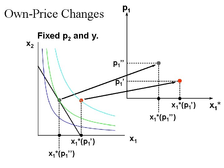
B. Own-Price Changes and the Demand Curve

The relationship between the quantity demanded of a good and its own price is perhaps the most famous in economics. The slope of the demand curve is related to the derivative $\frac{\partial x_i}{\partial p_i}$.

As we saw in the last lesson with the Slutsky equation, this derivative is composed of two parts:
$\frac{\partial x_i}{\partial p_i}=\underset{\text{Substitution Effect}}{\underbrace{\frac{\partial h_i}{\partial p_i}}}\underset{\text{Income Effect}}{\underbrace{-x_i\frac{\partial x_i}{\partial w}}}$

The substitution effect, $\frac{\partial h_i}{\partial p_i}$, is always non-positive. The sign of the income effect depends on whether the good is normal or inferior. This leads to two main possibilities for the total effect:

1. Ordinary Good: Demand falls when its price rises, $\frac{\partial x_i}{\partial p_i}<0$. This is the standard case, resulting in a downward-sloping demand curve. This always happens for normal goods (where the income effect is also negative, reinforcing the substitution effect) and for most inferior goods.
2. Giffen Good: Demand rises when its price rises, $\frac{\partial x_i}{\partial p_i}>0$. This is a rare case where a good is so strongly inferior that the positive income effect ($-x_i\frac{\partial x_i}{\partial w}$ becomes positive and outweighs the negative substitution effect. This results in an upward-sloping demand curve.

C. Cross-Price Changes: Substitutes and Complements

Finally, we can analyze how the demand for one good changes when the price of another good changes. This is measured by the cross-price derivative, $\frac{\partial x_i}{\partial p_j}$ for $i\ne j$.

• Goods $i$ and $j$ are gross substitutes if an increase in the price of good $j$ leads to an increase in the demand for good $i$: $\frac{\partial x_i}{\partial p_j}>0$. (e.g., coffee and tea).
• Goods $i$ and $j$ are gross complements if an increase in the price of good $j$ leads to a decrease in the demand for good $i$: $\frac{\partial x_i}{\partial p_j}<0$. (e.g., coffee and sugar).

The term "gross" is used because this definition is based on the Marshallian demand function, which includes both substitution and income effects. The Slutsky equation for cross-price effects, $\frac{\partial x_i}{\partial p_j}=\frac{\partial h_i}{\partial p_j}-x_j\frac{\partial x_i}{\partial w}$, shows that the income effect can sometimes complicate the relationship.

3. A Fundamental Property: Homogeneity

Marshallian demand functions have a crucial property: they are homogeneous of degree zero in all prices and income. Mathematically, this means:
$x_i(t\mathbf{p},tw)=t^0{x}_i(\mathbf{p},w)=x_i(\mathbf{p},w)\text{for any }t>0$
In words, if you scale all prices and income by the same positive factor $t$, the quantity demanded does not change. This is often called the principle of "no money illusion." A rational consumer's choices depend on real quantities—relative prices and real purchasing power—not on the nominal units of currency. Doubling all prices and your income doesn't make you any richer or poorer, and the relative trade-offs between goods remain the same, so your optimal consumption bundle should not change.

Let's see a proof of this property for the Cobb-Douglas case, which also serves as a great review of the properties we've just discussed.

4. Further Reading and Practice

To solidify these concepts, the following reading provides more examples and some excellent practice problems that directly test your understanding of comparative statics. Given your background, working through the calculus will be the best way to internalize the material.

Conclusion

Today we formalized the process of comparative statics in consumer theory. By taking partial derivatives of the Marshallian demand function $x_i(\mathbf{p},w)$, we can precisely predict how demand responds to changes in the economic environment.

Key Takeaways:

• Comparative statics is the analysis of how endogenous variables (like quantity demanded) respond to changes in exogenous variables (prices and income).
• The sign of $\frac{\partial x_i}{\partial w}$ determines if a good is normal or inferior and gives the slope of the Engel curve.
• The sign of $\frac{\partial x_i}{\partial p_i}$ determines if a good is ordinary or Giffen and gives the slope of the demand curve.
• The sign of $\frac{\partial x_i}{\partial p_j}$ determines if goods are gross substitutes or gross complements.
• Marshallian demand functions are homogeneous of degree zero in prices and income, meaning consumers are free from "money illusion."

Preview for the Next Lesson:
We have now thoroughly analyzed the consumer's optimal choice, $x_i(\mathbf{p},w)$. But what about the value the consumer gets from this choice? In the next lesson, we will construct and analyze the indirect utility function, $v(\mathbf{p},w)$, which tells us the maximum utility achievable at given prices and income, and revisit the expenditure function, $e(\mathbf{p},u)$. We will discover some powerful connections between these "value functions" and the demand functions we've been studying.