Monopoly Profit Maximization

Introduction

Welcome to our next lesson on monopoly. In our previous discussion, we established the defining characteristics of a monopoly, its sources of market power, and how that power is fundamentally constrained by the price elasticity of demand. We learned that unlike a competitive firm, a monopolist is a price-maker who can profitably charge a price above marginal cost.

Today, we will move from the conceptual to the computational. Your goal for this lesson is to learn how to calculate the profit-maximising price, output, and profit for a monopolist, given specific demand and cost functions. This process is the core of monopoly theory and involves a direct application of optimization principles. Given your background in statistics, the use of calculus to find this maximum should feel quite natural. The central rule we will derive and apply is that profit is maximized where marginal revenue equals marginal cost.

The Monopolist's Profit Maximization Rule

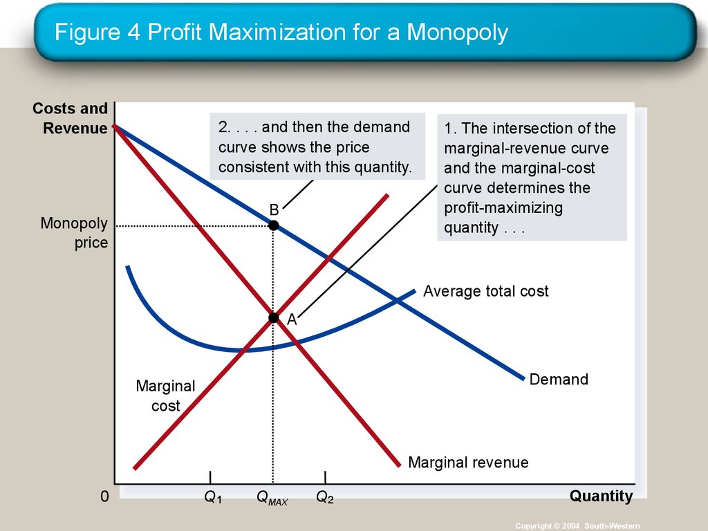
A monopolist, like any firm, maximizes profit by producing the quantity of output where marginal revenue (MR) equals marginal cost (MC).

MR = MC

The crucial difference between a monopolist and a perfectly competitive firm lies in the marginal revenue curve.

For a competitive firm, which is a price-taker, selling one more unit adds exactly the market price to its revenue. Therefore, $P = M R$ .
For a monopolist, which faces the entire downward-sloping market demand curve, selling one more unit requires lowering the price for all units sold. This means the revenue from the additional unit is less than the price it sells for. Therefore, for a monopolist, P > MR.

Deriving Marginal Revenue from Demand

Let's formalize this. This is a key analytical step that underpins all the calculations we will perform. Assume a linear inverse demand curve, which takes the general form:

P = a - b Q

Here, $a$ is the price-axis intercept and $- b$ is the slope.

Total Revenue (TR) is price times quantity:

T R = P \times Q = (a - b Q) Q = a Q - b Q^{2}

Marginal Revenue (MR) is the change in total revenue from selling one more unit, which we find by taking the first derivative of the total revenue function with respect to quantity $Q$ :

M R = \frac{d ( T R )}{d Q} = a - 2 b Q

Notice two critical features:

The MR curve has the same price-axis intercept ( $a$ ) as the demand curve.
The MR curve has twice the slope ( $- 2 b$ ) of the demand curve, meaning it is always steeper and lies below the demand curve (for $Q > 0$ ).

This "twice-as-steep" rule is a powerful shortcut for finding the marginal revenue curve when you are given a linear demand curve.

A Step-by-Step Guide to Calculating Monopoly Profit

To find the monopolist's optimal price, quantity, and profit, we follow a systematic, five-step process.

Find the Marginal Revenue (MR) function: Given the market demand curve, derive the MR function as shown above.
Find the Marginal Cost (MC) function: Given the firm's total cost (TC) function, find MC by taking the first derivative of TC with respect to $Q$ . $M C = \frac{d ( T C )}{d Q}$ .
Set MR = MC and solve for quantity ( $Q_{M}$ ): Equate the two functions and solve for the profit-maximizing quantity.
Find the monopoly price ( $P_{M}$ ): Substitute the optimal quantity $Q_{M}$ back into the inverse demand function ( $P = a - b Q$ ).
Calculate the profit ( $π$ ): Profit is Total Revenue minus Total Cost.
- Total Revenue: $T R = P_{M} \times Q_{M}$
- Total Cost: $T C (Q_{M})$ (substitute $Q_{M}$ into the original cost function)
- Profit: $π = T R - T C$

Let's look at the graphical representation of this process.

This graph illustrates the monopolist's profit-maximization decision. The profit-maximizing quantity (Q_MAX) is found at point A, where the Marginal Cost (MC) and Marginal Revenue (MR) curves intersect. The monopolist sets the price by finding the point on the Demand curve corresponding to this quantity (point B). Profit is the shaded area representing the difference between total revenue and total cost.

Worked Example: Two Approaches

Let's see this calculation in action. A video from "Economics in Many Lessons" provides an excellent walkthrough. It actually demonstrates two valid methods to solve the problem.

Method 1: Maximizing the Profit Function Directly
This approach involves writing the profit function, $π (Q) = T R (Q) - T C (Q)$ , and then finding the value of $Q$ that maximizes it by taking the derivative and setting it to zero.

Method 2: Equating MR and MC
This is the five-step process outlined above. As you'll see, the derivative of the profit function, $\frac{d π}{d Q}$ , is simply $M R - M C$ . Setting this to zero ( $M R - M C = 0$ ) is mathematically identical to setting $M R = M C$ .

Please watch the following two videos. The first shows the direct profit-maximization method, while the second uses the MR=MC rule for a slightly more complex cost function.

How to Find Monopoly Profit Maximizing Price, Quantity, and Profit

This video, "How to Find Monopoly Profit Maximizing Price, Quantity, and Profit," clearly demonstrates the direct optimization of the profit function. It's a great way to see the fundamental calculus at work.

Please watch the full video from start to finish. Notice how the profit function is constructed first, and then differentiated to find the optimal quantity.

Monopoly Profit Maximization with Calculus

This video, "Monopoly Profit Maximization with Calculus," applies the MR = MC rule. Pay attention to how MR and MC are derived separately before being equated. This example also uses a non-linear cost function, making MC dependent on quantity.

Watch the video segments that walk through the calculation step-by-step: First, see how to derive marginal revenue from the demand curve. Next, observe the derivation of marginal cost from the total cost function. Finally, watch how setting MR = MC yields the optimal quantity and then the price.

Practice with Problem Sets

Now that you've seen the methods, let's solidify your understanding by working through some typical exam-style problems. The following document contains a series of solved exercises. We will focus on two of them that illustrate common scenarios.

chapter 10 market power: monopoly and monopsony

This document provides several solved problems related to monopoly pricing. It's an excellent resource for practice and for seeing the theory applied in different contexts.

Please read through the detailed solutions for two specific exercises: Start with Exercise 4a (see problem). This is a classic case with a linear demand curve and a simple linear cost function, which means marginal cost is constant. Follow the steps: finding MR, finding MC, setting them equal to get Q, substituting Q into the demand curve for P, and finally calculating profit. Next, study Exercise 13a (see problem). This problem is more advanced, featuring a quadratic cost function (C = 100 - 5Q + Q^2). This means the marginal cost is no longer constant but increases with output. This is a more realistic scenario and a good test of your understanding of the general method.

By working through these examples, you'll see how the same five-step procedure can be applied regardless of the specific forms of the demand and cost functions. The key is the consistent application of the $M R = M C$ rule.

Conclusion

In this lesson, we have built a robust, quantitative framework for analyzing a monopolist's behavior. You have learned not just the profit-maximizing rule, but also the analytical steps required to apply it to concrete economic models.

Key Takeaways:

A monopolist maximizes profit by producing the quantity where Marginal Revenue (MR) equals Marginal Cost (MC).
For a monopolist, the MR curve is always below the demand curve because to sell more, the firm must lower its price on all units. For a linear demand curve $P = a - b Q$ , the marginal revenue is $M R = a - 2 b Q$ .
The calculation is a five-step process: find MR, find MC, set MR=MC to solve for Q, plug Q into the demand curve to find P, and finally calculate profit as $T R - T C$ .

You are now equipped to solve for the equilibrium outcome in a monopolistic market. In our next lesson, we will use these results to evaluate the social consequences of monopoly. We will calculate the consumer surplus, producer surplus, and deadweight loss to precisely measure the inefficiency that arises when a firm has market power.

Recommended resources