Profit Maximization in Perfect Competition

Introduction

Welcome to our next lesson. In our previous session, we established the foundational rule for profit maximization in a perfectly competitive market: a firm should produce at the quantity where the market price equals its marginal cost ( $P = M C$ ). This elegant simplification of the universal $M R = M C$ rule is the cornerstone of our analysis.

Today, we will put this rule into practice. Our objective is to calculate a competitive firm's short-run profit-maximizing output and the resulting economic profit. You will apply your quantitative skills to solve for these outcomes using two complementary methods: a graphical approach that builds intuition and an algebraic approach that provides precise solutions. We will work through several numerical problems, moving from basic cost functions to more complex scenarios, to ensure you are confident in applying these essential tools.

The Graphical Approach to Profit Maximization

Let's begin by visualizing the firm's decision. We can determine the optimal output and profit by combining the firm's cost curves with the market price line.

The process involves four straightforward steps:

Find the Optimal Quantity ( $q^{*}$ ): Locate the intersection of the horizontal price line ( $P = M R$ ) and the marginal cost ( $M C$ ) curve. This point gives you the profit-maximizing quantity, $q^{*}$ .
Find the Cost per Unit: At quantity $q^{*}$ , move vertically to the average total cost ( $A T C$ ) curve. The value on the vertical axis at this point is the cost per unit of production.
Calculate Profit per Unit: The difference between the price ( $P$ ) and the average total cost ( $A T C$ ) at $q^{*}$ is the profit (or loss) per unit.
Calculate Total Profit: Multiply the profit per unit by the quantity produced. This gives the total economic profit, $π$ . $π = (P - A T C) \times q^{*}$

This total profit can be visualized as the area of a rectangle on the graph.

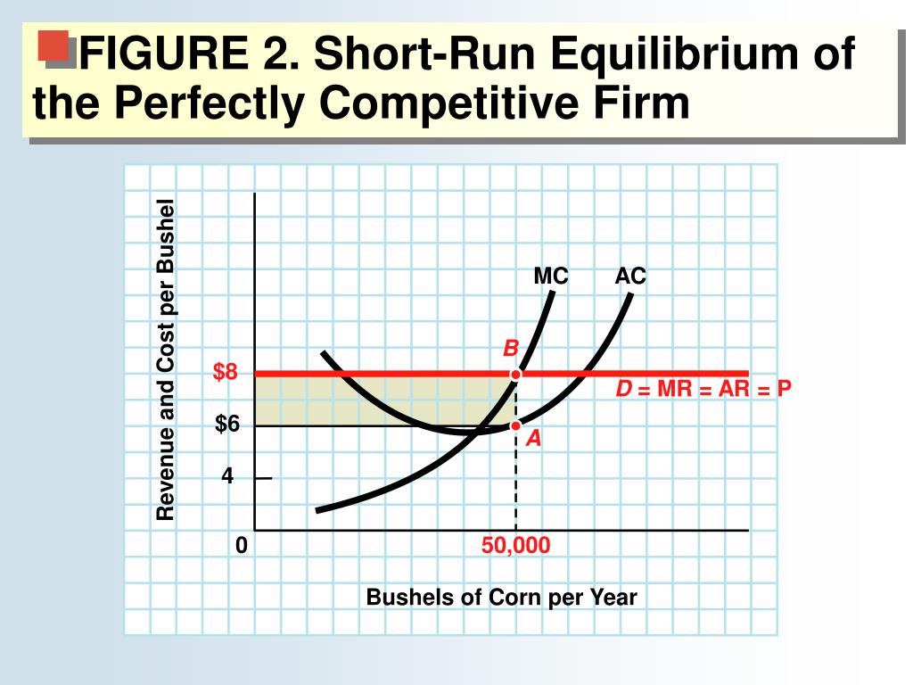
This graph illustrates a firm making a positive economic profit. The profit-maximizing quantity (50,000) is found where P (\$8) intersects MC. At this quantity, the ATC is \$6. The yellow shaded rectangle represents the total profit, with a height of (P - ATC) = (\$8 - \$6) = \$2 and a width of q = 50,000, for a total profit of \$100,000.

To see the complete calculation laid out with a graph, study the following resource.

1 Perfectly Competitive Markets

This document from UNC Charlotte provides a clear, step-by-step guide to finding the profit-maximizing output and profit from a firm's cost curve graph.

Please read the section titled The firm's picture and profit-maximization. Focus on the four steps outlined to find maximum profit using the graph with ATC, MC, and MR curves.

The Algebraic Method for Profit Maximization

While the graphical method is excellent for intuition, your background in statistics and mathematics makes the algebraic method a powerful and precise tool. This approach applies calculus to find the exact profit-maximizing quantity.

The firm's profit ( $π$ ) is total revenue ( $T R$ ) minus total cost ( $T C$ ):

π (q) = T R (q) - T C (q)

For a competitive firm, $T R (q) = P \cdot q$ , where $P$ is the constant market price. Thus:

π (q) = P \cdot q - T C (q)

To find the quantity $q$ that maximizes this function, we take the first derivative with respect to $q$ and set it to zero. This is the standard procedure for finding the maximum of a function.

\frac{d π}{d q} = \frac{d ( P \cdot q )}{d q} - \frac{d ( T C ( q ))}{d q} = 0

Since $P$ is a constant and the derivative of $T C (q)$ is $M C (q)$ , this gives us:

P - M C (q) = 0 ⟹ P = M C (q)

This confirms our rule. To find the optimal quantity $q^{*}$ , we solve the equation $P = M C (q)$ . Once we have $q^{*}$ , we can calculate the maximum profit by plugging it back into the profit function: $π = P \cdot q^{*} - T C (q^{*})$ .

Let's see this in action with a complete, worked-out example.

Perfect Competition: Profit Maximization (Problem #1)

This video from Economics in Many Lessons provides a clear, step-by-step walkthrough of a typical profit maximization problem, starting from a given price and a total cost function.

Watch the entire video from the beginning. Pay close attention to the sequence: Deriving the Marginal Cost function by differentiating the Total Cost function. Setting Price equal to Marginal Cost to solve for the optimal quantity, q. Calculating Total Revenue and Total Cost at the optimal quantity. Finally, computing the firm's profit.

Practice Problems and Variations

Now that you've seen the method, it's time to solidify your understanding by working through a variety of problems. The following video presents several scenarios that mirror the types of questions you might encounter.

Perfect Competition Example Problems: Algebra Based Solutions

This video, also from Economics in Many Lessons, contains a series of algebra-based problems that build on the core P=MC rule.

Please watch the following segments, focusing on the setup and solution for each problem: Problem 1 & 2 (Simple P=MC): These are straightforward applications where you are given P and a linear MC function. Problem 4 (Deriving P and calculating profit): This problem gives you TR and TC functions. You first have to deduce the market price from the TR function, then apply the P=MC rule and calculate the final profit. This is a comprehensive example. Problem 7 (Using Average Cost): This problem demonstrates how to calculate profit using the average cost function, connecting back to our graphical formula \pi = (P-AC) \times q. Note the result here: zero economic profit.

A Note on Economic Profit

An important point highlighted in the last video problem is the concept of zero economic profit. It's crucial to remember that we are always dealing with economic costs and profits, not accounting costs. A firm's total cost ( $T C$ ) function in economics includes all explicit costs (like wages and materials) and all implicit opportunity costs (like the income the entrepreneur could have earned elsewhere).

Therefore, when a firm earns zero economic profit, it is not a failure. It means that it is earning just enough revenue to cover all its explicit and implicit costs. This is considered a normal rate of return, making the venture worthwhile. A positive economic profit indicates an above-normal return.

This diagram shows a firm earning positive economic profit. The price (\$10) is greater than the average total cost (\$6) at the profit-maximizing output of 60 units. Total revenue is \$600, total cost is \$360, and the resulting economic profit is \$240.

Conclusion

In this lesson, we have moved from the theoretical rule of $P = M C$ to its practical application. You have learned how to calculate a perfectly competitive firm's profit-maximizing output and its corresponding profit or loss using both graphical and algebraic methods. The key is to first find the quantity where price equals marginal cost, and then compare the price to the average total cost at that quantity to determine the final profit.

Key Takeaways:

Profit-Maximizing Quantity ( $q^{*}$ ): Found by solving the equation $P = M C (q)$ .
Graphical Profit Calculation: The profit is the area of the rectangle defined by $(P - A T C) \times q^{*}$ .
Algebraic Profit Calculation: The profit is $π = T R (q^{*}) - T C (q^{*}) = P \cdot q^{*} - T C (q^{*})$ .
Economic Profit: This includes opportunity costs. Zero economic profit implies a normal rate of return and is the long-run equilibrium condition for this market, as we will see.

Our calculations today have shown firms making positive profits and zero profits. But what happens if the market price is so low that a firm makes a loss? Should it continue to produce at a loss or shut down operations entirely? This is the critical short-run decision we will analyze in our next lesson.

Recommended resources