Long-Run Equilibrium in Perfect Competition

The Dynamics of Long-Run Adjustment

The move from a short-run to a long-run equilibrium is driven by one simple motive: the pursuit of profit.

• Entry: If firms in a market are earning positive economic profits in the short run (i.e., Price > Average Total Cost), entrepreneurs will be attracted to this industry. New firms will enter the market. This entry increases the total number of sellers, which shifts the market supply curve to the right. As supply increases, the market price falls.
• Exit: Conversely, if firms are incurring losses (Price < Average Total Cost), some will find it unsustainable and exit the market. This exit reduces the number of sellers, shifting the market supply curve to the left. As supply decreases, the market price rises.

This process of entry and exit continues until a stable state is reached. This state, the long-run equilibrium, occurs when there is no longer any incentive for firms to enter or leave. This happens precisely when economic profit is zero.

The zero-profit condition gives us the fundamental equation for the long-run equilibrium. For profit ($\Pi$) to be zero:
$\Pi =TR-TC=0⟹TR=TC$
Dividing by quantity $q$, we get:
$\frac{TR}{q}=\frac{TC}{q}⟹P=ATC$
Since firms in perfect competition always produce where price equals marginal cost ($P=MC$) to maximize profit, the long-run equilibrium is characterized by a three-part condition:

Graphically, this occurs at the minimum point of the Average Total Cost (ATC) curve, where the MC curve intersects it. This is the firm's break-even point.

Calculating the Long-Run Equilibrium

Given the market demand and the cost structure of a typical firm, we can calculate all the key variables of the long-run equilibrium. The process involves a clear sequence of steps that leverages your quantitative skills.

Step 1: Find the Long-Run Output per Firm ($q_{LR}$)

The long-run equilibrium occurs where the firm produces at the lowest possible average total cost. As we know from the properties of cost curves, this is the quantity where MC = ATC.

1. Derive the Marginal Cost function, $MC(q)=\frac{dTC}{dq}$.
2. Derive the Average Total Cost function, $ATC(q)=\frac{TC(q)}{q}$.
3. Set $MC(q)=ATC(q)$ and solve for $q$. This is $q_{LR}$, the output level for each individual firm in the long run.

Step 2: Find the Long-Run Equilibrium Price ($P_{LR}$)

Since the long-run equilibrium condition is $P=MC=ATC$, we can find the market price by plugging the firm's long-run output ($q_{LR}$) into either the MC or the ATC function. Using the MC function is typically simpler.

1. Calculate $P_{LR}=MC(q_{LR})$.

This price is determined entirely by the cost structure of the firms. It is the lowest price at which firms can operate without making a loss.

Step 3: Find the Total Market Quantity ($Q_{LR}$)

The market price $P_{LR}$ must clear the market. To find out how much of the good consumers will buy at this price, we substitute $P_{LR}$ into the market demand equation.

1. Given the market demand function $Q_D=f(P)$, calculate $Q_{LR}=f(P_{LR})$.

Step 4: Find the Number of Firms in the Market ($n_{LR}$)

Finally, if the total market demand is $Q_{LR}$ and each identical firm is producing $q_{LR}$, the number of firms in the market is simply the total market output divided by the output per firm.

1. Calculate $n_{LR}=\frac{Q_{LR}}{q_{LR}}$.

Let's apply these steps to a concrete problem.

Example Walkthrough

Suppose a perfectly competitive market has a demand function given by $Q_d=24-P$. All firms in this market have an identical cost function: $C(q)=16+q^2$.

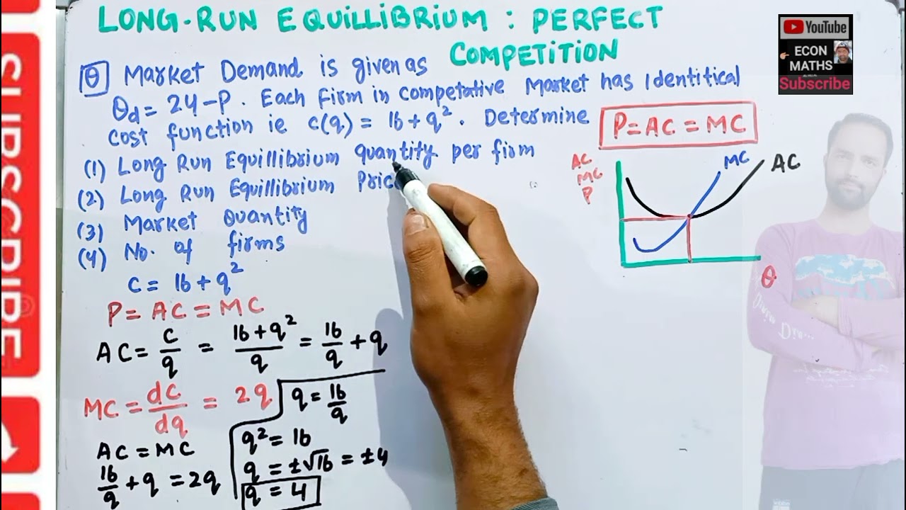
Let's follow our four steps:

1. Find Firm Output ($q_{LR}$):

   • First, derive MC and ATC. $$MC(q)=\frac{dC}{dq}=2q$$ $$ATC(q)=\frac{C(q)}{q}=\frac{16+q^2}{q}=\frac{16}{q}+q$$
   • Next, set $MC=ATC$. $$2q=\frac{16}{q}+q$$ $$q=\frac{16}{q}⟹q^2=16⟹q_{LR}=4$$

   Each firm will produce 4 units in the long run.

2. Find Market Price ($P_{LR}$):

   • Substitute $q_{LR}=4$ into the MC function. $$P_{LR}=MC(4)=2(4)=8$$

   The long-run market price will be $8.

3. Find Market Quantity ($Q_{LR}$):

   • Substitute $P_{LR}=8$ into the market demand function. $$Q_{LR}=24-P_{LR}=24-8=16$$

   The total market output will be 16 units.

4. Find Number of Firms ($n_{LR}$):

   • Divide total output by the output per firm. $$n_{LR}=\frac{Q_{LR}}{q_{LR}}=\frac{16}{4}=4$$

   In the long-run equilibrium, there will be 4 firms in the market.

This systematic approach allows you to solve for all the characteristics of a perfectly competitive market in the long run. The following video provides a comprehensive walkthrough of a similar problem, reinforcing these calculation steps.

For a rigorous, text-based derivation that you can refer back to, the following reading provides a similar, complete example.

An Alternative Method for Step 1

As a statistician familiar with optimization, you know that finding where $MC=ATC$ is equivalent to finding the minimum of the ATC curve. In the previous lesson, we found the minimum of the AVC curve by taking its derivative and setting it to zero. We can do the same here for ATC.

Alternative Step 1: Minimize ATC using Calculus

1. Derive the Average Total Cost function, $ATC(q)$.
2. Take the derivative of ATC with respect to $q$: $\frac{d(ATC)}{dq}$.
3. Set the derivative equal to zero and solve for $q$. This will give you $q_{LR}$.

Let's try this with our earlier example, where $ATC(q)=\frac{16}{q}+q$.

Setting this to zero:

This confirms our previous result for $q_{LR}$. Both methods are mathematically equivalent, and you can use whichever you find more intuitive. The following video demonstrates this calculus-based approach.

Conclusion

Today we've bridged the gap between the short run and the long run in perfectly competitive markets. We've seen how the engine of free entry and exit drives economic profits to zero, forcing firms to become as efficient as possible just to break even.

Key Takeaways:

• Long-Run Dynamics: Positive short-run profits attract new firms, increasing market supply and lowering prices. Losses cause firms to exit, decreasing supply and raising prices.
• Zero-Profit Condition: The long-run equilibrium is achieved when economic profits are zero.
• Equilibrium Condition: This occurs when a firm produces at the minimum of its average total cost curve, where $P=MC=ATC$.
• Calculation Procedure:
  1. Find the firm's output $q$ by setting $MC=ATC$.
  2. Find the market price $P$ by plugging $q$ into the MC function.
  3. Find the total market quantity $Q$ by plugging $P$ into the market demand function.
  4. Find the number of firms $n$ by calculating $Q/q$.

Having mastered the model of perfect competition, we are now ready to explore the opposite end of the market structure spectrum. In our next lesson, we will analyze the behavior of a monopoly—a single seller with the power to influence the market price. You will calculate how a monopolist's pricing and output decisions differ from those of a competitive firm and analyze the consequences for market efficiency.