Abatement Costs: Permits vs. Taxes

Introduction

In our last lesson, we concluded our analysis of specific market failures and interventions by examining how a price cap can compel a monopolist to increase output and reduce deadweight loss. We now turn to the final topic in this module: the problem of externalities, focusing on pollution.

When firms pollute, they impose costs on society that are not reflected in their private cost calculations. The goal of environmental policy is often to reduce pollution to a more socially optimal level. This lesson addresses a core question in policy design: if we need to achieve a certain total reduction in pollution across an industry, what is the most cost-effective way to do it?

Today, you will learn to calculate and compare the total costs of pollution abatement under three different policy regimes:

A "command-and-control" standard.
A corrective (Pigouvian) tax on emissions.
A system of tradeable emissions permits (cap-and-trade).

Building on your strong quantitative foundation, we will see that market-based instruments—taxes and permits—have a powerful advantage. They can achieve the desired environmental outcome at a lower total cost to society than a rigid standard by equalizing the marginal cost of abatement across all firms.

The Principle of Cost-Effective Abatement

Imagine an industry with two firms, A and B, that are both polluting. The government wants to reduce total pollution by 40 units. Each firm has a different technology and, therefore, a different cost structure for reducing its pollution. We model this with a Marginal Abatement Cost (MAC) curve for each firm, which represents the cost of reducing one additional unit of pollution.

Let's look at a graphical representation of this scenario.

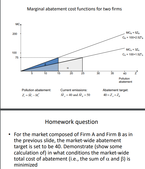
This graph shows the linear Marginal Abatement Cost (MAC) curves for two firms, A and B. The total cost of abating a certain amount `Z` is the area under the MAC curve up to that quantity (the triangles α and β).

The MAC functions are given as $M A C_{A} = 3 Z_{A}$ and $M A C_{B} = 5 Z_{B}$ , where $Z_{A}$ and $Z_{B}$ are the quantities of pollution abated by each firm. The government's target is $Z_{A} + Z_{B} = 40$ .

A simple approach might be to command each firm to abate an equal amount: $Z_{A} = 20$ and $Z_{B} = 20$ . Let's calculate the total cost of this policy.

The Total Abatement Cost (TAC) is the area under the MAC curve (a triangle with area $0.5 \times base \times height$ ).
$T A C_{A} = 0.5 \times Z_{A} \times M A C_{A} (20) = 0.5 \times 20 \times (3 \times 20) = 0.5 \times 20 \times 60 = $600$ .
$T A C_{B} = 0.5 \times Z_{B} \times M A C_{B} (20) = 0.5 \times 20 \times (5 \times 20) = 0.5 \times 20 \times 100 = $1000$ .
Total Cost (Standard): $600 + 1000 = $1600$ .

Notice that at this allocation, $M A C_{A} = 60$ while $M A C_{B} = 100$ . This means it costs Firm B $100 to reduce its last unit of pollution, while Firm A could have done it for only $60. This suggests an inefficiency. Society could save money by having Firm A abate a bit more and Firm B a bit less.

This leads us to the cost-effectiveness principle: the total cost of abatement is minimized if and only if the marginal abatement costs are equal for all firms.

M A C_{A} (Z_{A}) = M A C_{B} (Z_{B})

Let's solve for the cost-effective allocation:

Set MACs equal: $3 Z_{A} = 5 Z_{B}$ .
Use the total abatement constraint: $Z_{A} + Z_{B} = 40 ⟹ Z_{B} = 40 - Z_{A}$ .
Substitute and solve for $Z_{A}$ : $3 Z_{A} = 5 (40 - Z_{A}) ⟹ 3 Z_{A} = 200 - 5 Z_{A} ⟹ 8 Z_{A} = 200 ⟹ Z_{A} = 25$
Solve for $Z_{B}$ : $Z_{B} = 40 - 25 = 15$ .

Under this efficient allocation, the common marginal abatement cost is $3 \times 25 = $75$ (or $5 \times 15 = $75$ ). Now, let's calculate the new total cost:

$T A C_{A} = 0.5 \times 25 \times 75 = $937.50$ .
$T A C_{B} = 0.5 \times 15 \times 75 = $562.50$ .
Total Cost (Cost-Effective): $937.50 + 562.50 = $1500$ .

As you can see, by reallocating the abatement effort towards the lower-cost firm, the total cost of achieving the same environmental goal is reduced from $1600 to $1500.

Market-Based Policies: Taxes and Permits

The crucial insight is that we can design policies that lead firms to automatically choose this cost-effective outcome. The two primary market-based instruments are corrective taxes and tradeable permits. The following resource explains how they both work to achieve the same efficient result.

[PDF] Public bad: two firms in a market for a “pollutant”

This reference sheet formalizes the mechanisms for the policies we're discussing. It clearly explains why equalizing marginal abatement costs is efficient and how both taxes and permits achieve this.

Focus on these key parts: Read the section <span data-type="resource_reading_textrange" data-resource-subitem-id="6215b2d3" data-range-start="To find the optimal price" data-range-end="is equal to the Marginal Damages.">on aggregating MAC curves. Notice the process of horizontal summation: you rewrite each MAC function to express quantity (Z) in terms of price (MAC), and then add the quantities. 2. Then, study the section on the two policy solutions. Pay close attention to how both setting a tax (t = P*) and creating a cap-and-trade system lead to the same efficient outcome where each firm abates until its MAC equals the tax/permit price.

Let's briefly summarize how these policies would achieve the outcome from our example:

Corrective (Pigouvian) Tax: The regulator imposes a tax of $75 per unit of pollution.
- Firm A will reduce pollution as long as its MAC is less than the tax. It will stop at $M A C_{A} = 75 ⟹ 3 Z_{A} = 75 ⟹ Z_{A} = 25$ .
- Firm B will do the same: $M A C_{B} = 75 ⟹ 5 Z_{B} = 75 ⟹ Z_{B} = 15$ .
- The total abatement is $25 + 15 = 40$ , and the MACs are equalized. The policy works perfectly.
Tradeable Permits (Cap-and-Trade): The regulator caps total pollution and issues a corresponding number of permits. Firms can buy and sell these permits.
- If the total abatement target is 40, the market for permits will clear at a price that induces exactly 40 units of total abatement.
- This equilibrium price will be $75. Firms with low MAC (like Firm A) will find it cheaper to abate more and sell their spare permits, while firms with high MAC (like Firm B) will find it cheaper to buy permits than to abate.
- Trading continues until no firm can benefit from another trade, which occurs when all firms' MACs are equal to the permit price. The final allocation is $Z_{A} = 25$ and $Z_{B} = 15$ .

Both policies achieve the cost-effective allocation automatically, without the regulator needing to know each firm's individual cost structure—they only need to know the aggregate relationship between the price (tax/permit price) and the total quantity of abatement.

A Comprehensive Numerical Example

Now let's apply this framework to a more detailed problem. We will analyze a scenario from a solved exam question. This will allow us to cement the calculations for total abatement costs under different policies.

[PDF] 7 2) Suppose there is an industry with two firms. Currently Firm 1 is ...

This document contains a problem (Question 2) with two firms, a pollution reduction target, and asks for a comparison between a "fair" standard and a Pigovian tax. The provided solution key walks through the required calculations.

First, read Question 2 on page 7 to understand the setup. Then, carefully study the corresponding solution on page 10. Focus on how the total abatement costs are calculated for the "Standard" and "Tax" scenarios.

Let's reconstruct and verify the calculations from that resource.

Problem Setup:

Firm 1 Initial Emissions: 120 units. Marginal Savings from emitting: $M S_{1} = 120 - E_{1}$ .
Firm 2 Initial Emissions: 60 units. Marginal Savings from emitting: $M S_{2} = 120 - 2 E_{2}$ .
Socially optimal total emissions: 60 units.

First, let's translate the "Marginal Savings from Emitting" into the "Marginal Cost of Abating" framework, which is more direct for our purposes. Let $Z_{i}$ be the amount of pollution abated by firm $i$ . Abatement is the reduction from the initial level of emissions.

For Firm 1: Abatement $Z_{1} = 120 - E_{1}$ , so $E_{1} = 120 - Z_{1}$ . The MAC is the marginal savings foregone:
$M A C_{1} (Z_{1}) = 120 - E_{1} = 120 - (120 - Z_{1}) = Z_{1}$
For Firm 2: Abatement $Z_{2} = 60 - E_{2}$ , so $E_{2} = 60 - Z_{2}$ .
$M A C_{2} (Z_{2}) = 120 - 2 E_{2} = 120 - 2 (60 - Z_{2}) = 120 - 120 + 2 Z_{2} = 2 Z_{2}$

So we have a much simpler set of cost functions: $M A C_{1} = Z_{1}$ and $M A C_{2} = 2 Z_{2}$ .

The initial total emissions are $120 + 60 = 180$ . The target is 60 units.
Total Abatement Target: $Z_{1} + Z_{2} = 180 - 60 = 120$ units.

Scenario 1: "Fair" Standard

The policy commands each firm to emit half the social optimum: $E_{1} = E_{2} = 30$ .

Firm 1 abatement: $Z_{1} = 120 - 30 = 90$ units.
Firm 2 abatement: $Z_{2} = 60 - 30 = 30$ units.
Check: Total abatement is $90 + 30 = 120$ . The target is met.

Now, calculate the Total Abatement Cost (TAC) for each firm:

$T A C_{1} = \int_{0}^{90} Z_{1} d Z_{1} = [\frac{1}{2} Z_{1}^{2}]_{0}^{90} = 0.5 \times 9 0^{2} = 4050$ .
$T A C_{2} = \int_{0}^{30} 2 Z_{2} d Z_{2} = [Z_{2}^{2}]_{0}^{30} = 3 0^{2} = 900$ .
Total Cost (Standard): $4050 + 900 = $4950$ .
This matches the resource's calculation. At this point, $M A C_{1} = 90$ and $M A C_{2} = 2 \times 30 = 60$ . The costs are not equalized, so this is not cost-effective.

Scenario 2: Pigovian Tax / Tradeable Permits

To achieve the cost-effective outcome, we need to find the tax/permit price that induces 120 units of abatement. This occurs where $M A C_{1} = M A C_{2} = t$ .

From $M A C_{1} = t$ , we get $Z_{1} = t$ .
From $M A C_{2} = t$ , we get $2 Z_{2} = t ⟹ Z_{2} = t /2$ .

The total abatement must be 120:

Z_{1} + Z_{2} = 120 ⟹ t + t /2 = 120 ⟹ \frac{3}{2} t = 120 ⟹ t = \frac{2}{3} (120) = $80

So the optimal tax (or equilibrium permit price) is $80.

Now find the abatement levels and costs for each firm under this price:

Firm 1 abates: $Z_{1} = t = 80$ units.
Firm 2 abates: $Z_{2} = t /2 = 40$ units.
Check: Total abatement is $80 + 40 = 120$ . The target is met.

Calculate the TAC for each firm:

$T A C_{1} = 0.5 \times Z_{1}^{2} = 0.5 \times 8 0^{2} = 3200$ .
$T A C_{2} = Z_{2}^{2} = 4 0^{2} = 1600$ .
Total Cost (Tax/Permits): $3200 + 1600 = $4800$ .
This also matches the resource's calculation.

By using a market-based instrument, society achieves the same 120-unit reduction in pollution for $4800 instead of $4950, a saving of $150.

Conclusion

In this final lesson of our module on market failures, we have quantitatively demonstrated a fundamental principle of environmental economics: market-based instruments are more cost-effective than command-and-control regulations.

Key Takeaways:

Firms typically have different Marginal Abatement Cost (MAC) curves.
The cost-effective way to achieve a given total pollution reduction is to allocate abatement such that the MAC is equal across all firms.
A "command-and-control" standard that dictates a uniform abatement level for all firms generally fails to equalize MACs and is therefore not cost-effective.
Corrective (Pigouvian) taxes and tradeable permit systems (cap-and-trade) are two distinct policies that both create a price on pollution. They automatically lead profit-maximizing firms to adjust their abatement levels until their individual MAC equals this price, thus achieving the cost-effective outcome.
By calculating the total abatement cost (the sum of the areas under each firm's MAC curve), you can quantify the efficiency gains of using market-based instruments over rigid standards.

This lesson concludes our journey through microeconomic models of firms, markets, and government intervention. In our next lesson, we will pivot to the other major branch of economics, beginning our study of macroeconomics by learning how to measure the output of an entire economy.

Recommended resources