Deriving the IS Curve Algebraically

Goods Market Equilibrium: The Core Idea

The economy is in equilibrium when the total amount of output produced (Income, Y) is equal to the total amount of planned spending (Aggregate Demand, AD). For a closed economy with a government, aggregate demand is the sum of three components:

• Consumption (C): Spending by households.
• Investment (I): Spending by firms on capital and by households on new housing.
• Government Purchases (G): Spending by the government on goods and services.

The equilibrium condition is simply:

The "IS" in IS curve stands for "Investment" and "Saving." An alternative way to express this same equilibrium is that planned national saving equals planned investment. For today, we will focus on the $Y=C+I+G$ formulation.

The Graphical Derivation

Before we dive into the algebra, it's helpful to see the logic visually. The following classic diagram shows how the IS curve is derived from the relationship between the interest rate, investment, and aggregate demand.

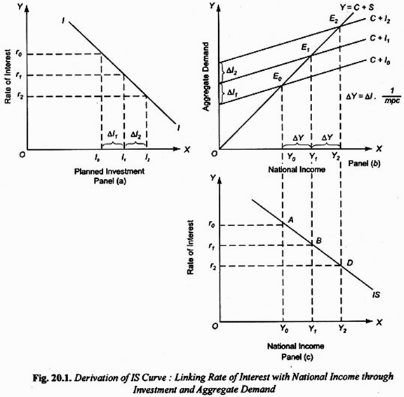
Let's break down what's happening in each panel:

1. Panel (a) - The Investment Function: This panel shows that planned investment (I) is negatively related to the rate of interest (r). When the interest rate falls from $r_0$ to $r_1$, it becomes cheaper for firms to borrow, so planned investment increases from $I_0$ to $I_1$.

2. Panel (b) - The Keynesian Cross: This diagram plots aggregate demand against national income. Equilibrium occurs where the AD line intersects the 45-degree line (where Y = AD). When the interest rate falls, investment increases by $\Delta I$. This shifts the entire aggregate demand curve upward (from $C+I_0$ to $C+I_1$). This higher demand leads, through a multiplier effect, to a larger increase in the equilibrium level of income, from $Y_0$ to $Y_1$.

3. Panel (c) - The IS Curve: This final panel simply plots the equilibrium points we've just identified. At interest rate $r_0$, the goods market is in equilibrium at income level $Y_0$ (point A). At the lower interest rate $r_1$, equilibrium income is $Y_1$ (point B). Connecting these points gives us the downward-sloping IS curve. It represents all pairs of (Y, r) where the goods market clears.

The Algebraic Derivation

Now, let's formalize this intuition with algebra, which will allow us to be much more precise. Our task is to find a single equation that relates Y and r, holding other factors constant.

We start with our equilibrium condition:

To make this useful, we need to substitute in specific functional forms for each component. These are called "behavioral equations" because they model the behavior of households and firms.

• Consumption (C): We assume consumption depends linearly on disposable income ($Y_D$). Disposable income is total income (Y) minus taxes (T). For now, let's assume a simple closed economy with no taxes, so $Y_D=Y$.

  $$C=a+bY$$

  Here, $a$ is autonomous consumption (spending that doesn't depend on income) and $b$ is the marginal propensity to consume (MPC), which is the fraction of an extra dollar of income that is spent.

• Investment (I): As seen in the graph, we model investment as having an autonomous component ($\bar{I}$) and a component that depends negatively on the real interest rate ($r$).

  $$I=\bar{I}-dr$$

  Here, $d$ is a parameter that measures how sensitive investment is to changes in the interest rate.

• Government Spending (G): We will treat government spending and taxes as exogenous, meaning they are fixed by policy and do not change when income or interest rates change. We denote them as $G=\bar{G}$ and $T=\bar{T}$.

The following video provides a clear, step-by-step derivation of the general IS equation using these components.

As the video shows, by substituting the behavioral equations into $Y=C+I+G$ and solving for Y, we arrive at the IS equation:

This equation explicitly defines the negative relationship between equilibrium income (Y) and the interest rate (r). The term $\frac{1}{1-b}$ is the familiar Keynesian multiplier.

A Numerical Example

Let's make this concrete by working through a numerical problem. This process of substituting values and solving for the equation is a core skill.

Suppose an economy is described by the following equations:

• Consumption: $C=40+0.5Y_D$
• Investment: $I=140-10r$
• Government Spending: $G=50$
• Taxes: $T=40$

The following video demonstrates how to derive the IS curve for a similar set of equations. Note that in this video's example, taxes are zero, so $Y_D=Y$. We will adapt the process for our case where taxes are present.

Now, let's solve our problem, which includes taxes.

1. Start with the equilibrium condition: $$Y=C+I+G$$
2. Substitute the behavioral equations: $$Y=(40+0.5(Y-T))+(140-10r)+50$$
3. Plug in the value for Taxes (T=40): $$Y=40+0.5(Y-40)+140-10r+50$$
4. Simplify and gather terms: $$Y=40+0.5Y-20+140-10r+50$$ $$Y=(40-20+140+50)+0.5Y-10r$$ $$Y=210+0.5Y-10r$$
5. Solve for Y by gathering Y terms on one side: $$Y-0.5Y=210-10r$$ $$0.5Y=210-10r$$
6. Isolate Y to get the final IS equation: $$Y=\frac{210}{0.5}-\frac{10}{0.5}r$$ $$Y=420-20r$$

This is the equation for our IS curve. For any given interest rate $r$, it tells us the level of income $Y$ that will clear the goods market. For example, if the interest rate is 5% (r=5), equilibrium income would be $Y=420-20(5)=320$.

Practice and Extension: Proportional Taxes

The model above used a "lump-sum" tax, where everyone pays a fixed amount. A more realistic scenario involves a proportional income tax, where taxes are a fraction ($t$) of income: $T=tY$. This changes the derivation slightly.

The following reading explains how to incorporate a proportional tax and provides another numerical example for you to review.

The key insight is that a proportional tax reduces the size of the multiplier. The new multiplier becomes $\frac{1}{1-b(1-t)}$, which is smaller than $\frac{1}{1-b}$. This means that any initial change in spending (from investment or government purchases) will have a smaller final impact on income, making the IS curve steeper.

Conclusion

Today we have formally derived the IS curve, which is a cornerstone of macroeconomic analysis. You've seen how it emerges both graphically and algebraically from the fundamental condition that production must equal planned spending in the goods market.

Key Takeaways:

• The IS curve represents all combinations of income (Y) and the interest rate (r) at which the goods market is in equilibrium.
• It is derived from the equation $Y=C+I+G$ by substituting behavioral functions for each component.
• The IS curve is downward-sloping because a lower interest rate stimulates higher investment, which in turn leads to a higher level of equilibrium income through the multiplier effect.
• The slope of the IS curve depends on the marginal propensity to consume (which determines the multiplier) and the interest sensitivity of investment.

In our next lesson, we will complete the other half of our model by algebraically deriving the LM curve, which represents equilibrium in the money market. Once we have both the IS and LM curves, we can put them together to find the single combination of income and the interest rate that brings the entire economy into simultaneous equilibrium.