Monopolistic Competition: Long-Run Equilibrium & Excess Capacity

The Transition from Short Run to Long Run

The story of the long run begins with short-run profits. When existing firms, like the pizza restaurant we analyzed previously, are making economic profits, it sends a signal to the market. Because there are no significant barriers to entry, new entrepreneurs will be attracted to the industry, hoping to capture a piece of the action.

What is the impact of these new entrants on an existing firm?

1. Decreased Demand: As more firms enter, a greater variety of substitute products becomes available. For an existing firm, this means it loses some of its market share. Its demand curve shifts to the left.
2. Increased Elasticity: With more close substitutes, consumers become more price-sensitive. A small price increase by one firm is more likely to send customers to a competitor. This makes the firm's demand curve more elastic (flatter).

This process of entry and the resulting leftward shift of the demand curve for incumbent firms will continue as long as economic profits remain positive. The market will only settle into a long-run equilibrium when the profit incentive disappears—that is, when firms are making zero economic profit.

The resource below provides an excellent graphical explanation of this adjustment process.

Calculating the Long-Run Equilibrium

The long-run equilibrium is defined by two simultaneous conditions:

1. Profit Maximization: The firm must be doing the best it can, which means producing the quantity where $MR=MC$.
2. Zero Economic Profit: The incentive for entry or exit must be gone, which means profit is zero. This occurs where $P=ATC$.

Graphically, this happens at the unique point where the demand curve is tangent to the ATC curve. At this exact quantity, the MR curve will intersect the MC curve.

This provides a clear procedure for solving these problems mathematically, which leverages your analytical skills. A firm's cost structure (specifically its fixed costs) must be compatible with its demand curve for this zero-profit tangency to occur. Let's work through a quantitative example.

Excess Capacity: The Price of Variety

A significant consequence of the long-run equilibrium in monopolistic competition is the presence of excess capacity. Let's examine the graph of this equilibrium.

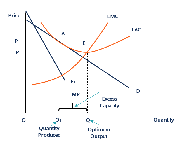
As you can see, the zero-profit tangency point (where $P=ATC$) occurs on the downward-sloping portion of the average total cost curve. This is a mathematical necessity when the demand curve itself is downward-sloping. This means the firm produces a quantity ($Q_1$ in the graph) that is less than the quantity that would minimize its average total cost ($Q$ in the graph).

Excess Capacity is defined as the difference between the minimum-cost output and the actual long-run equilibrium output.

Excess Capacity = $Q_{\text{efficient scale}}-Q_{\text{long run}}$

To quantify this, you need to calculate two different output levels:

1. The Long-Run Equilibrium Output ($Q_{LR}$): This is the quantity we found in the previous section, where the firm maximizes profit and makes zero profit.
2. The Efficient Scale Output ($Q_{eff}$): This is the quantity that minimizes the Average Total Cost (ATC). As we learned in a previous module, the MC curve intersects the ATC curve at its minimum point. Therefore, you can find this quantity by setting $MC=ATC$.

This "inefficiency" is often described as the price we pay for product diversity. If all firms produced at their minimum ATC, their products would be more standardized. The market offers variety, but at the cost of each firm operating at a slightly smaller, less-efficient scale. Your experience designing unique apparel items, rather than mass-producing a single generic design, illustrates this trade-off perfectly.

A Graphical Application

Let's apply these concepts to interpret a graph that shows the transition from short run to long run.

This graph shows the demand and MR curves for a firm initially ("Demand Initial", "MR Initial") and after market entry has occurred ("Demand Later", "MR Later"). Let's analyze it step-by-step, as if it were an exam question.

a. Short-run equilibrium ("Initial" state):

1. Profit-maximizing output: Find where MR Initial intersects MC. This occurs at Q = 8 units.
2. Price: At Q=8, go up to Demand Initial. The price is P = $10.
3. Profit per unit: At Q=8, the ATC is approximately $7.50. So, profit per unit is $10-7.50=\$2.50$.
4. Total profit: $(\text{Price}-\text{ATC})\times Q=(\$2.50)\times 8=\$20$.

b. Long-run equilibrium ("Later" state):

1. Profit-maximizing output: Find where MR Later intersects MC. This occurs at Q = 6 units.
2. Price: At Q=6, go up to Demand Later. The price is P = $9.
3. Profit per unit: At Q=6, the Demand Later curve is tangent to the ATC curve. This means $P=ATC$, so profit per unit is $9-9=\$0$.
4. Total profit: $0.

c. What happened to this industry?
The firm was initially earning a $20 economic profit. This attracted new firms to the market. The entry of competitors, offering similar but differentiated products, reduced the original firm's demand, shifting its demand curve from Demand Initial to Demand Later. This process continued until the demand curve became tangent to the ATC curve, at which point economic profits were eliminated, and the incentive for new firms to enter disappeared. The market reached its long-run equilibrium.

Conclusion

In this lesson, we traced the path of a monopolistically competitive firm from earning short-run profits to settling into a long-run equilibrium. The mechanism of free entry is the key driver of this adjustment.

Key Takeaways:

• Short-run economic profits attract new entrants, which shifts the demand curve of existing firms to the left.
• The long-run equilibrium is reached when Price equals Average Total Cost ($P=ATC$), meaning economic profits are zero.
• At this equilibrium, the firm is still maximizing profit, so the $MR=MC$ condition also holds.
• Because the downward-sloping demand curve is tangent to the ATC curve, the firm produces at an output level to the left of the minimum ATC.
• This gives rise to excess capacity, which can be quantified as the difference between the efficient-scale output (where $MC=ATC$) and the long-run equilibrium output.

We have now seen markets with many small firms (perfect competition) and many small-but-differentiated firms (monopolistic competition). Our next lesson will shift focus to oligopoly, a market structure dominated by a few large firms. This scarcity of competitors introduces a new and fascinating element: strategic interdependence, where each firm's decisions depend critically on the anticipated actions of its rivals. To analyze this, we will need to add a new tool to our quantitative toolkit: game theory.