Output Gaps and the Business Cycle

Introduction

In our last lesson, we explored the Phillips curve and established that while a short-run trade-off exists between inflation and unemployment, the long-run Phillips curve is vertical at the natural rate of unemployment ( $u_{n}$ ). This natural rate represents an equilibrium where inflation is stable because the labor market is neither "too tight" nor "too slack."

Today, we will extend this concept of a long-run equilibrium from the labor market to the economy's overall production. We will introduce potential output, which is the level of production corresponding to the natural rate of unemployment. This lesson will equip you to define potential output, calculate the output gap, and identify phases of the business cycle from data. By comparing the economy's actual output to its potential, we gain a crucial diagnostic tool for assessing economic health and anticipating inflationary pressures, much like how the unemployment gap ( $u_{t} - u_{n}$ ) informed our analysis of the Phillips curve.

Defining Potential Output and the Output Gap

An economy's output, as measured by real GDP, fluctuates over time. To understand these fluctuations, we need a benchmark. This benchmark is known as potential output or potential GDP.

It's crucial to understand that potential output is not the absolute physical maximum an economy could produce. Instead, it is the highest level of output that can be sustained over the long term without generating upward pressure on inflation. It's the level of output an economy produces when all its resources—labor and capital—are employed at their normal, sustainable rates. This directly corresponds to the economy operating at the natural rate of unemployment ( $u_{n}$ ).

To understand the core definitions, please read the following brief sections from an article by the St. Louis Federal Reserve.

Minding the Output Gap: Potential GDP & Why It Matters

This article provides clear, non-technical definitions of the core concepts for this lesson.

Please read the introductory paragraphs up to the first heading, from the definition of Real GDP. Then, read the section titled "What Is Potential Output?". Finally, jump to the end of the article to review the definitions provided for Potential output and Actual output.

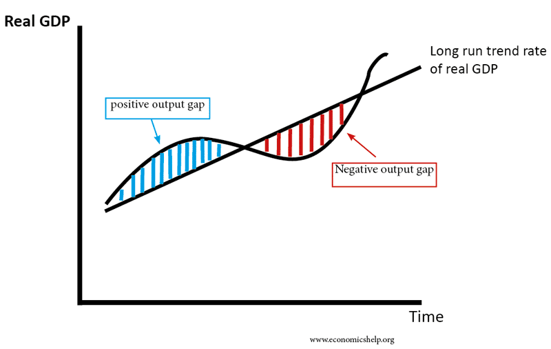
The difference between the economy's actual output and its potential output is called the output gap. It's a key indicator of the economy's position in the business cycle.

There are two types of output gaps:

Negative Output Gap (or Recessionary Gap): This occurs when Actual Output < Potential Output. The economy is underperforming, with idle resources. This corresponds to a situation where unemployment is above its natural rate ( $u_{t} > u_{n}$ ). This slack in the economy tends to put downward pressure on inflation.
Positive Output Gap (or Inflationary Gap): This occurs when Actual Output > Potential Output. The economy is "overheating," with resources being used at an unsustainable rate. This corresponds to unemployment being below its natural rate ( $u_{t} < u_{n}$ ). This strain on resources tends to fuel inflation.

The following video provides a concise explanation of these concepts.

Output Gaps

This video from EconplusDal, "Output Gaps," clearly defines and illustrates the two types of gaps.

Watch the first segment for a clear definition of the output gap and its negative form. Then, skip to the section that defines a positive output gap. The video also shows how these gaps are represented in the AD-AS model, which we will study in detail in a later module.

The Business Cycle

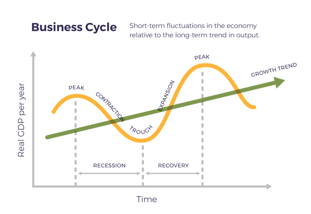
The output gap is the defining feature of the business cycle, which describes the short-term fluctuations of actual real GDP around the long-term trend of potential GDP. These fluctuations occur in a repeating, though not perfectly regular, pattern of phases:

Expansion (or Recovery): A period where real GDP is growing. The output gap is narrowing (if negative) or becoming positive.
Peak: The high point of an expansion, where real GDP is at its highest level before a downturn. The output gap is typically positive.
Contraction (or Recession): A period where real GDP is falling. A recession is often formally defined as two consecutive quarters of negative real GDP growth. The output gap is becoming negative or more negative.
Trough: The low point of a contraction, where real GDP is at its lowest level before an upturn begins. The output gap is at its most negative point.

The following diagrams visually represent these concepts. The first shows the idealized phases of the business cycle, while the second explicitly labels the positive and negative output gaps.

An illustration of the business cycle, showing the phases of expansion, peak, contraction, and trough as fluctuations of real GDP around a long-term growth trend.

This graph shows how the deviation of real GDP from its long-run trend creates positive output gaps (when actual GDP is above trend) and negative output gaps (when it is below trend).

Calculating the Output Gap

Now, let's turn to the quantitative application. The output gap is most usefully expressed as a percentage of potential GDP. As a statistician, you can think of this as normalizing the deviation by the scale of the economy.

The formula, as noted in the St. Louis Fed article, is:

Percentage Output Gap = \frac{Actual GDP - Potential GDP}{Potential GDP} \times 100%

Let's work through an example. Consider the following data for a hypothetical economy:

Year	Actual GDP ($ Billions)	Potential GDP ($ Billions)
2020	19,500	20,000
2021	20,400	20,500
2022	21,525	21,000
2023	21,420	21,500
2024	22,000	22,000

We can calculate the output gap for each year and identify the state of the economy.

2020:
- Gap = $19, 500 - 20, 000 = - 500$
- % Gap = $\frac{- 500}{20 , 000} \times 100% = - 2.5%$
- State: Negative output gap (Recessionary Gap). The economy is in a contraction/recession.
2021:
- Gap = $20, 400 - 20, 500 = - 100$
- % Gap = $\frac{- 100}{20 , 500} \times 100% \approx - 0.49%$
- State: Negative output gap, but closing. The economy is in an expansion/recovery phase.
2022:
- Gap = $21, 525 - 21, 000 = + 525$
- % Gap = $\frac{+ 525}{21 , 000} \times 100% = + 2.5%$
- State: Positive output gap (Inflationary Gap). The economy is overheating, likely near a peak.
2023:
- Gap = $21, 420 - 21, 500 = - 80$
- % Gap = $\frac{- 80}{21 , 500} \times 100% \approx - 0.37%$
- State: Negative output gap. The economy has entered a contraction after the peak in 2022.
2024:
- Gap = $22, 000 - 22, 000 = 0$
- % Gap = $0%$
- State: No output gap. The economy is operating at its full potential.

The Challenge of Estimating Potential Output

A critical point that your background in statistics will help you appreciate is that potential output is an unobserved variable. We can observe actual GDP, but potential GDP must be estimated. This estimation is a major challenge for economists and policymakers and is subject to significant uncertainty and revision.

Estimating potential output is fundamentally a problem of signal extraction: decomposing the time series of real GDP into a long-run trend component (the "signal," or potential output) and a cyclical component (the "noise," or the output gap).

Economists use several methods for this:

Statistical Methods: These approaches use filters to smooth the historical real GDP data to extract a trend. A well-known example is the Hodrick-Prescott (HP) filter, which balances the smoothness of the trend with its closeness to the actual data. These are purely data-driven.
Structural Methods: These approaches use economic theory, typically a production function, to build up an estimate of potential output from estimates of the sustainable levels of labor, capital, and total factor productivity.

For a deeper, though still high-level, look at these different estimation techniques, you may find the following research paper from the Reserve Bank of Australia insightful.

[PDF] Estimating Output Gaps - Reserve Bank of Australia

This paper provides a sophisticated overview of the methods economists use to estimate the unobservable concept of potential output. It is more advanced than required for your exam, but it directly engages with the statistical challenges of this topic.

Focus on the Introduction, which frames the problem. Then, skim the descriptions of the five methods in Section 2, starting from the main heading. Pay attention to the names of the methods (Linear, Hodrick-Prescott, Multivariate HP, Unobservable Components, Production Function) and the brief conceptual description of each, rather than the detailed mathematics. This will give you a strong sense of the analytical rigor and the inherent uncertainty involved.

Policy Implications: Closing the Gap

Policymakers at central banks and in governments monitor the output gap closely because it signals inflationary pressures and labor market conditions. A persistent negative gap means lost output and high unemployment, while a persistent positive gap creates unsustainable inflation.

Therefore, a primary goal of macroeconomic policy is to minimize the size and duration of output gaps, keeping the economy operating close to its potential.

When there is a negative (recessionary) gap, policymakers use expansionary policy (e.g., lower interest rates, increased government spending, or tax cuts) to boost aggregate demand and close the gap.
When there is a positive (inflationary) gap, they use contractionary policy (e.g., higher interest rates, decreased government spending, or tax increases) to cool down the economy.

The following video from Khan Academy provides an excellent quantitative example of how fiscal policy (changes in government spending or taxes) can be used to close an output gap. This will serve as a good review of the multiplier concepts we've covered previously.

Calculating change in spending or taxes to close output gaps | AP Macroeconomics | Khan Academy

This video, "Calculating change in spending or taxes to close output gaps," walks through the math of using fiscal policy to steer the economy back toward its potential.

First, watch the introductory section which reviews the concepts of inflationary and recessionary gaps and the corresponding policy responses. Then, follow the numerical example of closing a negative output gap by increasing government spending. Note how the spending multiplier, which depends on the Marginal Propensity to Consume (MPC), determines the size of the required policy action.

The key insight from the video's calculation is that an initial change in government spending has a magnified impact on total output, determined by the multiplier $1/ (1 - MPC)$ . To close a $100 billion output gap with an MPC of 0.75, the required spending increase is only $25 billion, because the multiplier is 4. This is a powerful demonstration of how these theoretical concepts guide real-world policy decisions.

Conclusion

This lesson has bridged the gap between our analysis of labor market equilibrium and the broader macroeconomy. By defining potential output as the sustainable production level consistent with the natural rate of unemployment, we have developed a powerful framework for diagnosing the economy's health.

Key Takeaways:

Potential Output is the maximum sustainable level of real GDP, achieved when the economy is at its natural rate of unemployment.
The Output Gap is the percentage deviation of actual GDP from potential GDP.
A negative (recessionary) gap implies idle resources and unemployment above its natural rate, putting downward pressure on inflation.
A positive (inflationary) gap implies an overheating economy and unemployment below its natural rate, creating upward pressure on inflation.
The business cycle describes the fluctuation of actual GDP around potential GDP through phases of expansion, peak, contraction, and trough.
Calculating the output gap is a crucial first step for policymakers in deciding whether to use expansionary or contractionary policy to stabilize the economy.

This lesson concludes our module on Macroeconomic Indicators and Objectives. We have now defined and learned to calculate the core metrics used to measure economic performance: GDP, inflation, and unemployment, and explored the key relationships between them.

In our next module, we will begin our study of International Trade and Finance. We will shift our focus from a single, closed economy to an open one, exploring how countries interact through trade and financial flows. We will start by examining the fundamental question of why nations trade and how to calculate the gains from specialization.

Recommended resources