Peak-Load Pricing: Optimal Price Calculation

Introduction

In our previous lesson, we analyzed how a firm can increase its profits by charging different prices to different groups of customers through third-degree price discrimination. We'll now extend this idea of differential pricing to a different context: time. Many firms face demand that fluctuates predictably over time (e.g., higher during the day than at night, or on weekends than weekdays) while being constrained by a fixed production capacity.

This lesson addresses the learning outcome of calculating optimal prices under a peak-load pricing scheme with differing demand conditions. We will explore the strategic problem faced by firms like electricity providers, hotels, and airlines. You will learn the analytical framework to determine the profit-maximizing prices for both "peak" and "off-peak" periods, a decision that hinges on the interplay between variable costs, capacity costs, and the capacity constraint itself. Given your strong quantitative background, we will ground this in a formal optimization problem.

The Peak-Load Pricing Model

At its core, peak-load pricing is a form of intertemporal price discrimination. The firm sets different prices for the same service at different points in time. The key distinction from our previous models is the presence of a fixed production capacity, which is costly to build and cannot be exceeded in the short run.

To understand how prices are set, we must first distinguish between two types of costs:

Variable Cost ( $c$ ): The cost of producing one additional unit of output, assuming capacity is available. For an electric company, this is the fuel cost. For a hotel, it's the cost of cleaning a room. We'll assume this is constant per unit.
Capacity Cost ( $r$ ): The cost of creating one additional unit of capacity. For an electric company, this is the cost of building more power plant infrastructure. For a hotel, it's the cost of building another room. This cost must be paid regardless of whether the capacity is used.

The firm's problem is to choose an optimal capacity level, $K$ , and then set a price for the peak period ( $P_{1}$ ) and a price for the off-peak period ( $P_{2}$ ) to maximize total profit.

The following reading from an MIT economics course provides an excellent conceptual overview of this problem.

[PDF] 1 2. Optimal Wholesale Pricing and Investment in Generation

This document provides a clear, intuitive explanation of peak-load pricing. It was written to be accessible but maintains economic rigor.

Please read Section 2, "The Simplest Peak-Load Pricing Story". Pay close attention to the distinction between variable cost (c) and capacity cost (r), and how the model determines the optimal prices in the "Off-peak and On-peak Prices" subsection. The logic here is the foundation for our calculations.

The Formal Pricing Rules

As the reading explains, the optimal pricing strategy depends on whether the capacity constraint is binding. Let's formalize this. A profit-maximizing firm faces two distinct demand curves: $D_{1}$ for the peak period and $D_{2}$ for the off-peak period, with corresponding marginal revenue curves $M R_{1}$ and $M R_{2}$ .

The firm's profit ( $π$ ) is the sum of revenues from both periods, minus the total variable costs and the total capacity cost:

π = [P_{1} (Q_{1}) \cdot Q_{1}] + [P_{2} (Q_{2}) \cdot Q_{2}] - c (Q_{1} + Q_{2}) - r K

This is maximized subject to the constraints that output in either period cannot exceed capacity: $Q_{1} \leq K$ and $Q_{2} \leq K$ .

The solution to this constrained optimization problem, which can be formally derived using methods like Kuhn-Tucker optimization, yields two key scenarios.

Scenario 1: Off-Peak Demand Does Not Use Full Capacity

This is the most common case. The firm builds enough capacity to satisfy peak demand, and the off-peak demand is not large enough to fill this capacity.

Off-Peak Period: Since capacity is not a constraint, the firm behaves like a standard monopolist. It produces until the marginal revenue from off-peak customers equals the marginal cost of producing one more unit. Here, the relevant marginal cost is just the variable cost, $c$ .
$M R_{2} = c$
The firm finds the quantity $Q_{2}$ that satisfies this, and sets the price $P_{2}$ from the off-peak demand curve $D_{2}$ .
Peak Period: In the peak period, demand is high enough that the firm produces at full capacity, so $Q_{1} = K$ . The price $P_{1}$ is determined by what the peak-demand customers are willing to pay for that quantity $K$ . But how is $K$ determined? In the long run, the firm will increase capacity as long as the marginal revenue from doing so in the peak period covers both the variable cost ( $c$ ) and the capacity cost ( $r$ ).
$M R_{1} = c + r$
This equation determines the optimal capacity $K$ , and the peak price $P_{1}$ is then found from the peak demand curve $D_{1}$ at $Q_{1} = K$ . Essentially, the peak users pay for the entire cost of the capacity.

To see a more rigorous derivation of these results, the following paper uses the mathematical optimization framework you're familiar with.

[PDF] Peak Load Pricing: An Illustration through Kuhn-Tucker

This paper formalizes the peak-load pricing model as a constrained optimization problem.

Focus on the "MODEL" section to understand the setup of the profit maximization problem. Then, read "Case I", which derives the pricing rules for the common scenario where the off-peak constraint is non-binding. This directly corresponds to the logic we just discussed.

Worked Example: A Graphical Approach

Let's apply these rules to a typical exam-style problem. The graph below shows a firm's demand curves for peak ( $D_{1}$ ) and off-peak ( $D_{2}$ ) periods, their marginal revenue curves ( $M R_{1}, M R_{2}$ ), and the firm's short-run marginal cost ( $M C_{S R}$ ).

This graph shows the demand and marginal revenue curves for a peak period (D1, MR1) and an off-peak period (D2, MR2). The firm's short-run marginal cost (MC_SR) is horizontal at \$10 up to a capacity of 4,000 units, at which point it becomes vertical, indicating a capacity constraint.

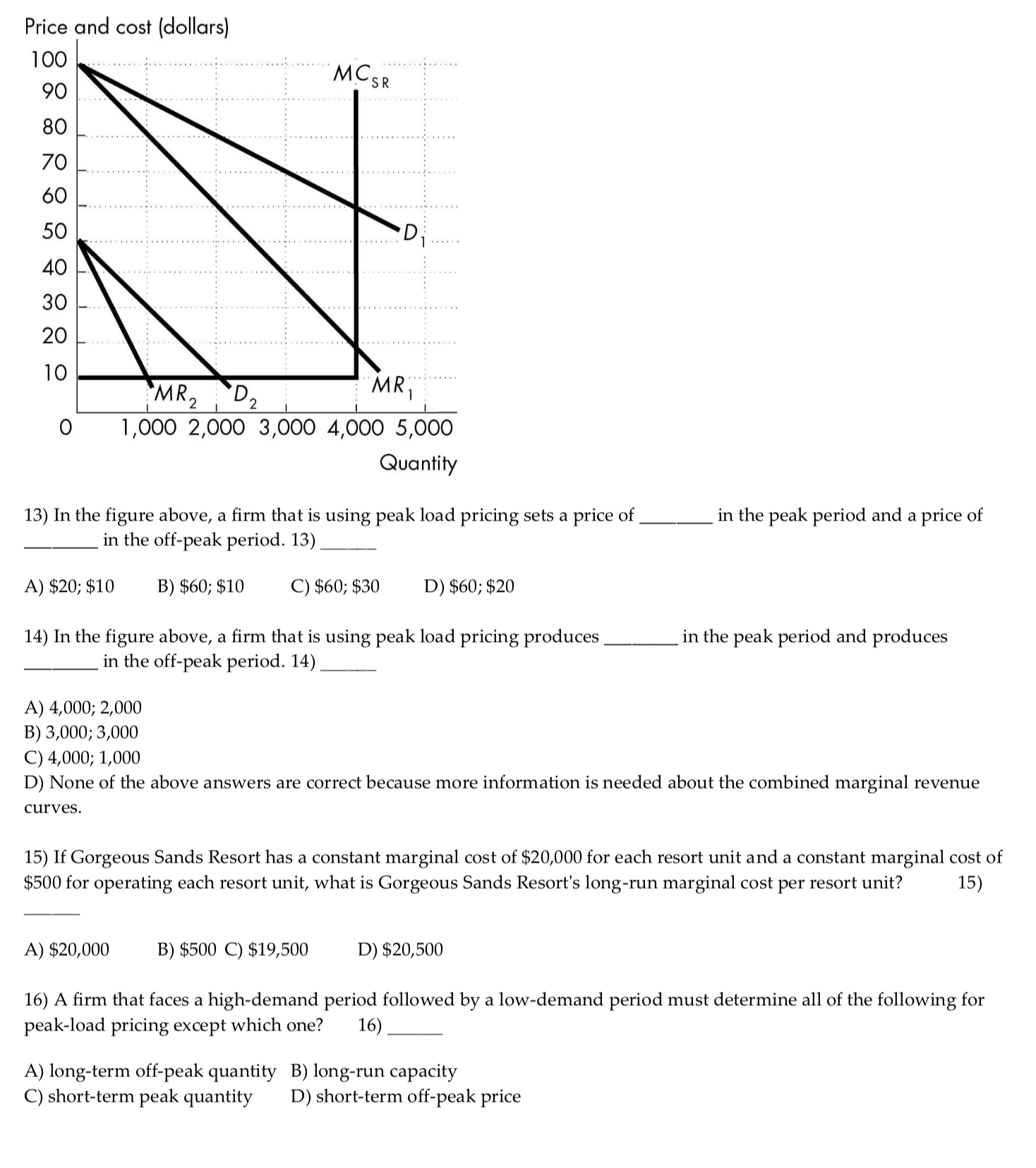
From this graph, we can deduce:

The variable cost, $c$ , is the constant marginal cost up to capacity, so $c = $10$ .
The capacity, $K$ , is the quantity where the marginal cost becomes vertical, so $K = 4, 000$ units.

Now, let's calculate the optimal prices and quantities.

1. Off-Peak Period (Demand $D_{2}$ )
We apply the rule $M R_{2} = c$ .

Find the intersection of the $M R_{2}$ curve and the marginal cost of $10.
This occurs at a quantity of $Q_{2} = 2, 000$ units.
To find the price, we move up from $Q_{2} = 2, 000$ to the off-peak demand curve, $D_{2}$ .
The corresponding price on the vertical axis is $P_{2} = $30$ .

Notice that $Q_{2} = 2, 000 < K = 4, 000$ , confirming this is the "non-binding" scenario.

2. Peak Period (Demand $D_{1}$ )
In the peak period, the firm will sell up to its capacity limit.

The quantity sold is $Q_{1} = K = 4, 000$ units.
To find the price, we move up from $Q_{1} = 4, 000$ to the peak demand curve, $D_{1}$ .
The corresponding price on the vertical axis is $P_{1} = $60$ .

Summary of Results:

Peak Period: Price = $60, Quantity = 4,000
Off-Peak Period: Price = $30, Quantity = 2,000

This analysis directly answers questions 13 and 14 accompanying the image. The correct price combination is $60 (peak) and $30 (off-peak), and the quantity combination is 4,000 (peak) and 2,000 (off-peak).

Scenario 2: Off-Peak Demand is Binding

What if demand in the off-peak period is also very high? It's possible for the capacity constraint to be binding in both periods. This would happen if, at a price that covers variable cost, off-peak users wanted more than the capacity $K$ .

In this case, the firm produces $Q_{1} = Q_{2} = K$ . The pricing rule changes because now both sets of customers contribute to the cost of capacity. The capacity cost $r$ is shared between them. The formal condition from the Kuhn-Tucker analysis is:

(M R_{1} - c) + (M R_{2} - c) = r

This states that the marginal profit contribution from the last unit of capacity sold in the peak period, plus the marginal profit contribution from that same unit in the off-peak period, must equal the marginal cost of that unit of capacity. This is a more advanced case, but the logic flows directly from the constrained optimization framework. You can read about this in "Case II" of the Gulati & Kaur paper you reviewed earlier.

Conclusion

This lesson has equipped you with the analytical tools to solve peak-load pricing problems. You can now calculate the optimal prices and quantities for a firm with fixed capacity and fluctuating demand, a common and important pricing strategy.

Key Takeaways:

Peak-load pricing is used by firms with fixed, costly capacity and demand that varies over time.
The pricing structure depends on two costs: a per-unit variable cost ( $c$ ) and a per-unit capacity cost ( $r$ ).
In the standard case, the off-peak quantity is determined by setting $M R_{o f f - p e ak} = c$ .
The firm's capacity ( $K$ ) is set to serve peak demand, where $M R_{p e ak} = c + r$ . The peak price is then the price consumers are willing to pay at quantity $K$ .
Graphically, you can find the off-peak price by finding where $M R_{2}$ intersects the variable cost line, and the peak price by finding the price on $D_{1}$ at the capacity limit.

In our next lesson, we will shift our focus from pricing based on demand characteristics to pricing based on strategic interactions with potential rivals. We will start by examining limit pricing, a strategy used by incumbent firms to deter new competitors from entering the market.

Recommended resources