Understanding and Computing Covariance and Correlation Matrices

1. Understanding Covariance: The Direction of Movement

Before we can understand how two assets move together, we need to recall how we measure the movement of a single asset. That measure is variance, which quantifies how much an asset's returns are spread out from their average.

Covariance extends this idea to two assets. It measures the directional relationship between their returns. Do they tend to move in the same direction, or in opposite directions?

To build a strong intuition for this, let's start with a video that explains the concept visually.

As the video explained, the covariance formula essentially checks if, on average, the returns of two assets are on the same side of their respective means at the same time.

The key takeaway is the sign of the covariance:

• Positive Covariance: The two assets tend to move in the same direction. (e.g., Google and Microsoft).
• Negative Covariance: The two assets tend to move in opposite directions. (e.g., an airline stock and an oil stock).
• Zero Covariance: There is no linear relationship between their movements.

However, covariance has a significant drawback: its magnitude is hard to interpret. A large covariance value could mean a strong relationship, or it could simply be because the assets themselves are very volatile (i.e., have large return values). This lack of standardization makes it difficult to compare the relationships between different pairs of assets.

2. Correlation: Adding Strength to Direction

To solve the interpretation problem of covariance, we use correlation. Correlation normalizes covariance, scaling the value to a bounded range of -1 to +1.

$\text{Correlation}(X,Y)=\frac{\text{Covariance}(X,Y)}{{\sigma }_x\cdot {\sigma }_y}$

Where ${\sigma }_x$ and ${\sigma }_y$ are the standard deviations of the returns for Asset X and Asset Y. By dividing by the product of the individual standard deviations, we effectively remove the scale of the assets' volatility, leaving us with a pure measure of their linear relationship.

This video segment explains the transition from covariance to correlation.

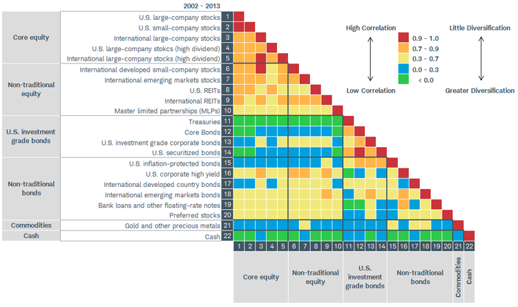
The correlation matrix is the result of this calculation for all pairs of assets in a portfolio:

• Its values range from -1 to +1.
• The diagonal is always 1, as an asset is perfectly correlated with itself.
• A value close to +1 indicates a strong positive relationship (bad for diversification).
• A value close to -1 indicates a strong negative relationship (excellent for diversification).
• A value close to 0 indicates no linear relationship (good for diversification).

3. Computing Covariance and Correlation in Python

Now let's move to the practical part. As a quant developer, you'll most often perform these calculations using libraries like pandas and NumPy.

Using pandas and seaborn

The pandas library is incredibly convenient for this task, especially when you start with a DataFrame of asset prices. The workflow is typically:

1. Load prices into a DataFrame.
2. Calculate a DataFrame of returns using .pct_change().
3. Calculate the covariance matrix with .cov().
4. Calculate the correlation matrix with .corr().
5. Visualize the correlation matrix using a heatmap from the seaborn library for quick interpretation.

This entire workflow is covered in the next video.

Using NumPy and Manual Calculation

While pandas is convenient, understanding the NumPy implementation is also valuable, especially given your CS background. It connects more directly to the underlying linear algebra. You can compute the matrices directly from a NumPy array of returns.

For a deeper understanding of the formulas and their implementation, the following resource is excellent. It not only shows the NumPy functions but also walks through a manual calculation, which solidifies the concepts.

import pandas as pd
import seaborn as sns
import matplotlib.pyplot as plt

data = {
    'NVDA': [0.02, -0.01, 0.03, 0.015],
    'AMD': [0.018, -0.012, 0.025, 0.013],
    'INTC': [-0.005, 0.002, -0.008, 0.001]
}
returns_df = pd.DataFrame(data)

import pandas as pd
import seaborn as sns
import matplotlib.pyplot as plt

data = {
    'NVDA': [0.02, -0.01, 0.03, 0.015],
    'AMD': [0.018, -0.012, 0.025, 0.013],
    'INTC': [-0.005, 0.002, -0.008, 0.001]
}
returns_df = pd.DataFrame(data)

# 1. Calculate the correlation matrix
correlation_matrix = returns_df.corr()
print("Correlation Matrix:\n", correlation_matrix)

# Interpretation:
# 2. Most correlated pair: NVDA and AMD have a correlation of ~0.998,
#    meaning they move almost perfectly in sync.

# 3. Best diversification: Both NVDA and AMD have a strong negative
#    correlation with INTC (~ -0.95), making INTC a good candidate to
#    diversify a portfolio holding either of the other two.

# 4. (Optional) Create a heatmap
plt.figure(figsize=(6, 4))
sns.heatmap(correlation_matrix, annot=True, cmap='coolwarm', vmin=-1, vmax=1)
plt.title('Stock Correlation Matrix')
plt.show()

Conclusion

In this lesson, we demystified the covariance matrix that we used in the previous lesson. You now have a solid conceptual and practical understanding of both covariance and correlation, which are central to modern portfolio theory and risk management.

Key Takeaways:

• Covariance measures the directional relationship between assets' returns but is difficult to interpret due to its scale-dependency.
• Correlation is a standardized measure (-1 to +1) of the direction and strength of a linear relationship, making it far more useful for comparing pairs of assets.
• For portfolio diversification, the goal is to combine assets with low or, ideally, negative correlation to reduce overall portfolio volatility.
• In Python, you can easily compute these matrices using pandas (.cov(), .corr()) or NumPy (np.cov(), np.corrcoef()).
• Visualizing the correlation matrix with a heatmap is a standard and highly effective way to quickly assess relationships within a universe of assets.

Preview of the Next Lesson:

We are about to shift gears from statistics to calculus. The next lesson, "Define a derivative as a rate of change and relate it to the concept of financial 'Greeks'," will introduce a new fundamental concept. While correlation helps us understand historical relationships between assets, derivatives and the 'Greeks' will help us measure an instrument's instantaneous sensitivity to changes in market factors like stock price, time, and volatility. This is essential for pricing and hedging options.