Calculating Technical Debt Proxy Scores

Introduction

In our last two lessons, you've done some excellent work engineering features from two different data sources. First, you extracted process metrics from Git history to quantify development activity. Then, you computed aggregate flakiness features from test execution logs to measure test stability.

Today, we complete our feature engineering trifecta by turning our attention to the source code itself. Our learning outcome is to calculate technical debt proxy scores from static analysis output. You'll learn how to take the raw findings from code analysis tools and transform them into quantitative scores that represent different facets of technical debt.

This is a cornerstone for your goal of building a technical debt prioritization tool. The scores you'll learn to calculate today can serve as the direct target for a machine learning model—the very thing you want to rank and prioritize.

What is Technical Debt, and How Can We Measure It?

You've likely heard the term "technical debt" used to describe messy, hard-to-maintain code. The metaphor is powerful: taking shortcuts now is like taking on debt, which you'll have to pay back later with "interest" in the form of slowed development, more bugs, and increased maintenance costs.

To build a prioritization tool, we need to move beyond this qualitative feeling and assign concrete numbers to debt. Let's explore the most common methods for doing this.

As you've just read, there isn't one single way to calculate technical debt. Instead, we have a toolkit of different "proxy scores," each suited for a different purpose:

• Technical Debt Ratio (TDR): A high-level financial metric perfect for business discussions. It compares the cost to fix the code versus the cost to build it.
• Code-Based Remediation Cost (e.g., SQALE): A bottom-up, time-based estimate. This is highly actionable for engineering teams as it represents the total person-hours needed to fix all known issues.
• Maintainability Index (MI): A single score (often 0-100) based on metrics like complexity and lines of code, giving a quick-glance assessment of code health.
• Hotspot Analysis: Identifies high-risk files by combining code complexity with change frequency (which you learned to calculate in a previous lesson!).

For our project, the Code-Based Remediation Cost is often the most useful, as it provides a direct, quantifiable measure of effort that we can use for prioritization.

From Theory to Practice: Static Analysis Output

These formulas rely on data generated by static analysis tools. These tools scan your source code without executing it, checking for thousands of predefined rules related to bugs, vulnerabilities, and "code smells" (indicators of deeper problems).

SonarQube is a very popular tool for this. Let's look at what its output actually looks like.

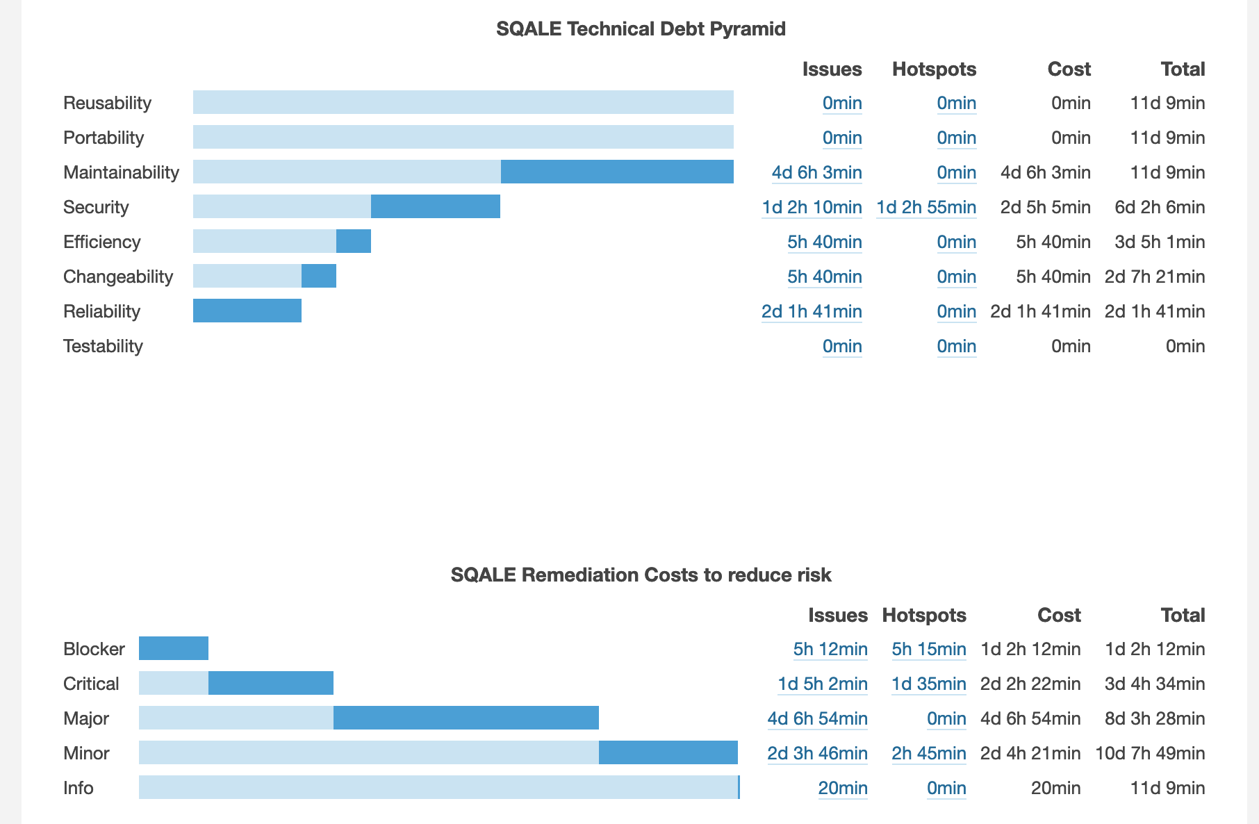
To understand how these numbers are derived, it's helpful to look at the tool's own definitions.

From the reading, we can see the core logic used by SonarQube:

1. Every detected issue (a "code smell") has a pre-configured remediation cost in minutes (e.g., "fixing this complex method will take 30 minutes").
2. The total Technical Debt (sqale_index) is simply the sum of the remediation costs of all issues. This is our "principal."
3. The Technical Debt Ratio (sqale_debt_ratio) is then calculated using this principal, giving us a percentage score.

A Step-by-Step Calculation Example

Let's make this concrete by walking through a calculation, combining the concepts from both resources. We'll calculate the TDR for a hypothetical project.

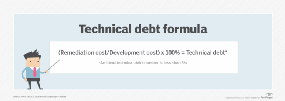
Step 1: Establish Initial Development Cost

This is the denominator of our TDR formula. Let's assume our project cost $500,000 to build.

Step 2: Quantify the Remediation Cost (The "Principal")

We run a static analysis tool like SonarQube on our codebase. It scans the code and produces a report. Let's say it finds:

• 1,500 "Minor" issues, each estimated at 10 minutes to fix.
• 200 "Major" issues, each estimated at 30 minutes to fix.
• 50 "Critical" issues, each estimated at 60 minutes to fix.

The total remediation effort in minutes is:
(1500 * 10) + (200 * 30) + (50 * 60) = 15,000 + 6,000 + 3,000 = 24,000 minutes.

This is our sqale_index. To convert it to a monetary cost, we use a blended developer rate (e.g., $90/hour).

Total Remediation Effort (hours) = 24,000 / 60 = 400 hours.
Remediation Cost (RC) = 400 hours * $90/hour = $36,000.

Step 3: Calculate the Technical Debt Ratio (TDR)

Now we plug our numbers into the formula:

Our TDR is 7.2%. This score is a powerful proxy for technical debt that can be tracked over time.

Here's how you'd do that final calculation in Python:

remediation_cost = 36000
development_cost = 500000

tdr = (remediation_cost / development_cost) * 100

print(f"The Technical Debt Ratio (TDR) is: {tdr:.1f}%")

From Raw Analysis to a Feature Matrix

For your ML project, you'll want to calculate these scores on a more granular level (e.g., per file or per module). Imagine you've exported the raw issue list from your static analysis tool into a CSV. You can use Pandas to aggregate this data into proxy scores.

Let's assume the raw data looks like this:

import pandas as pd




# Sample raw output from a static analysis tool
data = {
    'file_path': [
        'auth/user.py', 'auth/user.py', 'auth/session.py',
        'payment/core.py', 'payment/core.py', 'payment/utils.py'
    ],
    'severity': ['Major', 'Minor', 'Minor', 'Critical', 'Major', 'Minor'],
    'remediation_minutes': [30, 10, 5, 60, 30, 15]
}
issues_df = pd.DataFrame(data)

print("--- Raw Static Analysis Output ---")
print(issues_df)

Now, let's calculate two proxy scores for each file: the total remediation time (debt_minutes) and the number of issues (issue_count).

# Group by file_path and aggregate
debt_per_file = issues_df.groupby('file_path').agg(
    debt_minutes=('remediation_minutes', 'sum'),
    issue_count=('remediation_minutes', 'size')
)

print("\n--- Technical Debt Proxy Scores per File ---")
print(debt_per_file)

This debt_per_file DataFrame is exactly what you need! The debt_minutes column is a direct proxy for the "pain" associated with each file. In a technical debt prioritization tool, you would use a model to predict or rank files based on this score, combined with other features you've engineered.

Conclusion

In this lesson, you've bridged the gap between the abstract idea of "bad code" and the concrete, numerical scores needed to build an ML-powered tool.

Key Takeaways:

• Technical debt can be quantified using proxy scores derived from static analysis output.
• Common methods include calculating the Technical Debt Ratio (TDR), total Remediation Cost (in time or money), and a Maintainability Index.
• Static analysis tools like SonarQube generate these scores by identifying code smells and summing up their predefined remediation times.
• Using Python and Pandas, you can aggregate raw issue reports from these tools to calculate debt scores on a per-file or per-module basis, creating features ready for an ML model.

Preview of the Next Lesson:
You have now engineered features from three distinct sources: Git history (process), test logs (execution), and now source code (static analysis). Each provides a unique perspective on code quality. In the next lesson, "Assemble engineered features into a structured feature matrix," you will learn how to combine all of these different features into a single, unified dataset, preparing it for the model training stage.