Introduction
Welcome to the third module of our course, where we will dive into the powerful world of data transformation. In the previous modules, you built a solid foundation by setting up your R environment, learning to work with RStudio Projects, and mastering the full cycle of importing, inspecting, and exporting data. You can now confidently bring data into R and save your work, which are essential skills for any analysis.
This lesson introduces a concept that is central to modern data analysis in R: the pipe operator (%>%). Your goal is to learn how to use this operator to chain dplyr functions into a clear, readable, and efficient workflow. Think of the pipe as the grammar that connects the "verbs" of data manipulation you'll learn throughout this module. Mastering the pipe will fundamentally change how you write and think about your R code, making it more intuitive and powerful.
1. The Challenge of Complex Operations
Before we introduce the solution, let's consider the problem. Imagine you need to perform several sequential steps to clean or analyze a dataset. For example, in a clinical trial dataset, you might want to:
- Filter for patients in a specific treatment group.
- Select only the columns related to patient ID and symptom scores.
- Arrange the results to show patients with the highest scores first.
Without a dedicated tool, there are two common ways to write this code, neither of which is ideal.
Method 1: Creating Intermediate Objects
You could save the result of each step into a new variable.
# Step 1: Filter the data
filtered_data <- filter(raw_data, treatment_group == "A")


# Step 2: Select columns from the filtered data
selected_data <- select(filtered_data, patient_id, symptom_score)


# Step 3: Arrange the selected data
final_data <- arrange(selected_data, desc(symptom_score))
This approach works, but it clutters your R environment with temporary variables (filtered_data, selected_data) that you don't need to keep. For a long analysis, this becomes messy and hard to manage.
The video "How to use pipes in dplyr" by the channel thatRnerd explains this exact problem.
Watch the segment from the beginning to see a demonstration of how creating multiple intermediate variables can make your workflow cumbersome.
Method 2: Nesting Functions
Alternatively, you could nest the function calls inside one another.
final_data <- arrange(select(filter(raw_data, treatment_group == "A"), patient_id, symptom_score), desc(symptom_score))
This avoids creating extra variables, but it's very difficult to read. You have to work from the inside out to understand the sequence of operations, which is counter-intuitive. Keeping track of parentheses becomes a chore, and debugging is a nightmare.
2. The Solution: The Pipe Operator %>%
The Tidyverse provides an elegant solution to this problem: the pipe operator, written as %>%. This operator allows you to write code that is both clean and easy to read from left to right, just like a sentence.
The pipe comes from the magrittr package (and is a core part of the tidyverse), inspired by the work of artist René Magritte, famous for his painting of a pipe titled "The Treachery of Images."
The %>% operator takes the output of the expression on its left and passes it as the first argument to the function on its right. You can read it out loud as "and then".
Let's revisit our three-step example, this time using the pipe:
final_data <- raw_data %>%
  filter(treatment_group == "A") %>%
  select(patient_id, symptom_score) %>%
  arrange(desc(symptom_score))
This code reads naturally: "Take raw_data, and then filter it, and then select columns, and then arrange the result." This structure is far more readable and easier to write and debug.
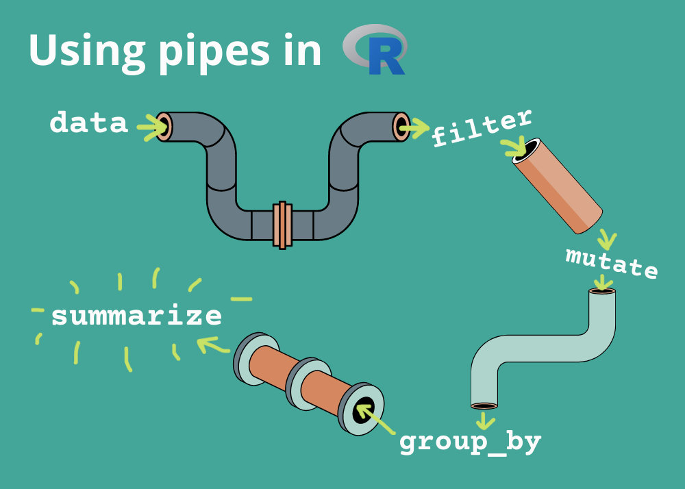
Introducing the Pipe Operator in R
The video "Introducing the Pipe Operator in R" from the Duke Center for Computational Thinking provides a fantastic conceptual overview using a "morning routine" analogy.
Please watch the entire video from start to finish. It will help you build a strong mental model of what the pipe does and why it's so powerful for readability. Pay close attention to how it compares piped code to nested code.
3. How the Pipe Works with dplyr
The dplyr package is designed with the pipe in mind. Every major dplyr function (which we'll call "verbs") takes a data frame as its first argument. This is precisely why the pipe works so seamlessly with them.
When you write data %>% some_function(argument2), R interprets it as some_function(data, argument2). The pipe automatically handles passing the data frame to the next function in the chain.
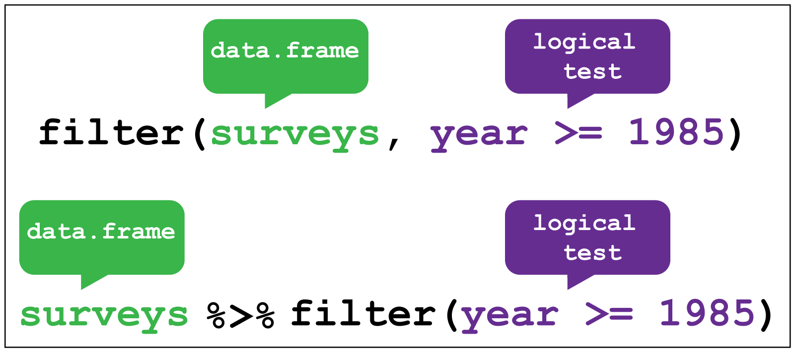
The reading below offers another great analogy (making pancakes!) and demonstrates how to combine simple dplyr verbs into a pipeline.
Chapter 4 Pipes and dplyr: the easy way of data manipulation
This chapter from "Machine learning in R" provides a great introduction to the pipe and how it connects dplyr verbs.
First, read the section on "R pipes", focusing on the pancake story to solidify your intuition. Then, jump to the section "Basics of dplyr package" and read the short example comparing nested functions to a piped approach using select() and head().
As you saw, the piped version is structured in the same order that the operations are executed, making it far easier to follow the logic. In RStudio, you can use the keyboard shortcut Ctrl + Shift + M (Windows/Linux) or Cmd + Shift + M (macOS) to insert the %>% operator.
4. Let's Practice
Time to put this into practice. Open your clinical-trial-practice RStudio Project and create a new R script named 07-pipe-operator.R.
We'll use the built-in mtcars dataset for this exercise. It contains data on fuel consumption and 10 other aspects of car design and performance for 32 automobiles.
-
Load packages and data. Add this code to your script to load the
tidyverseand view themtcarsdata.library(tidyverse) # mtcars is built-in, so we can use it directly. # We'll work with a copy to be safe. cars_data <- mtcars # View the data to get familiar with it glimpse(cars_data) -
The "Before" Code (Nested Functions). Here is a sequence of operations written using the messy nested style. This code finds all cars with 6 cylinders (
cyl == 6), selects only the columns for miles per gallon (mpg), horsepower (hp), and weight (wt), and finally arranges them by horsepower in descending order.Copy this code into your script, run it, and look at the
heavy_6cyl_carsdata frame.# Nested approach (hard to read) heavy_6cyl_cars <- arrange( select( filter(cars_data, cyl == 6), mpg, hp, wt ), desc(hp) ) View(heavy_6cyl_cars) -
Your Task: Rewrite with Pipes. Now, it's your turn. Below the previous code block, rewrite the same sequence of operations using the
%>%operator. Save the result to a new object calledheavy_6cyl_cars_piped.Hint: Start with
cars_data %>% ...and add each function call on a new line.Click here to see the solution
# Piped approach (easy to read)
heavy_6cyl_cars_piped <- cars_data %>%
  filter(cyl == 6) %>%
  select(mpg, hp, wt) %>%
  arrange(desc(hp))

View(heavy_6cyl_cars_piped)
If you run
View(heavy_6cyl_cars_piped), you should see the exact same result asheavy_6cyl_cars, but your code is now structured logically and is much more readable.
This exercise demonstrates the core value of the pipe: it transforms hard-to-read, nested code into a clear, step-by-step recipe for data manipulation.
Conclusion
In this lesson, you've been introduced to one of the most important operators in the Tidyverse, the pipe (%>%). By creating logical, sequential workflows, the pipe addresses the common problems of code readability and complexity that arise from nested functions or excessive temporary variables. This is the foundational skill for all the data transformation work we will do from now on.
Key Takeaways:
- The pipe operator
%>%takes the result from its left side and passes it as the first argument to the function on its right. - You can read
%>%as "and then," which helps articulate the flow of data through your analysis. - Piping allows you to chain multiple
dplyrfunctions together into a single, readable sequence, avoiding nested code and temporary variables. - The keyboard shortcut
Ctrl+Shift+MorCmd+Shift+Mis a convenient way to type the pipe operator.
Preview of the Next Lesson:
Now that you understand the "grammar" of dplyr workflows, we will start learning the "verbs." In the next lesson, you will master select() and rename(), the two primary functions for choosing, removing, and renaming columns in your data frames.