Good to continue. In the last lesson, you used context managers to give files and other external resources a reliable lifetime. Here the focus shifts from resource scope to numerical work: moving repeated arithmetic out of the Python interpreter and into NumPy array operations.
This is a foundational habit for AI engineering. Image tensors, token features, normalization statistics, attention masks, and embedding batches are all arrays with meaningful shapes. By the end of this lesson, you should be able to translate an element-wise nested loop into a broadcasted NumPy expression, predict its output shape, and recognize when broadcasting would create an unreasonably large intermediate result.
From a mathematical rule to an array operation
Consider a batch of feature vectors:
where is batch size and is feature width. Suppose we want to add one learned bias value to each feature position:
Here . The same vector is applied to every example in the batch.
A direct Python implementation is correct:
import numpy as np


def add_bias_loop(
    features: np.ndarray,
    bias: np.ndarray,
) -> np.ndarray:
    batch_size, width = features.shape

    if bias.shape != (width,):
        raise ValueError(
            f"expected bias shape {(width,)}, got {bias.shape}"
        )

    result = np.empty(
        features.shape,
        dtype=np.result_type(features, bias),
    )

    for batch_index in range(batch_size):
        for feature_index in range(width):
            result[batch_index, feature_index] = (
                features[batch_index, feature_index]
                + bias[feature_index]
            )

    return result
But the loops are not expressing the important idea. The computation is simply “add the feature bias to every row.” NumPy can express that directly:
def add_bias(
    features: np.ndarray,
    bias: np.ndarray,
) -> np.ndarray:
    return features + bias
The numerical result is identical. The difference is where the iteration happens:
- In the first version, Python executes an operation for every pair.
- In the second version, NumPy dispatches an element-wise operation over contiguous numerical buffers using compiled low-level code.
This is vectorization: writing the operation over arrays rather than explicitly indexing individual scalar elements. Broadcasting is the shape rule that makes features + bias meaningful even though the inputs have shapes and .
Be precise about one related distinction:
elementwise = features * weights
matrix_product = features @ weights
* uses element-wise semantics and may use broadcasting. @ performs matrix multiplication, which combines and sums over an axis. Do not replace a matrix product with * merely because both operations involve two arrays.
Learn NumPy broadcasting in 6 minutes! 📡
Watch “Learn NumPy broadcasting in 6 minutes!” from Bro Code for a compact visual introduction to shape compatibility.
Watch the core rule for the purpose of broadcasting, then continue through worked shapes. Focus on the fact that dimensions are compared from right to left, not from the first axis forward.
The broadcasting rule: align shapes from the right
For element-wise NumPy operations, align the two shapes at their rightmost ends. Each aligned pair of dimensions is compatible if:
- the dimensions are equal, or
- one of them has size .
If one input has fewer dimensions, treat its missing leading dimensions as size .
For our bias example:
| Array | Actual shape | Shape after conceptual alignment |
|---|---|---|
features |
||
bias |
||
| result | — |
The dimension of size in the conceptual shape expands across the batch dimension. So each row receives the same bias.
For concrete arrays:
features = np.array(
    [
        [0.2, 1.0, -0.5],
        [0.7, 0.1, 2.0],
    ],
    dtype=np.float32,
)

bias = np.array([0.1, -0.2, 0.3], dtype=np.float32)

shifted = features + bias

print(shifted)
# [[ 0.3  0.8 -0.2]
#  [ 0.8 -0.1  2.3]]

print(shifted.shape)
# (2, 3)
The supplied illustration shows exactly this row-wise application of a vector.
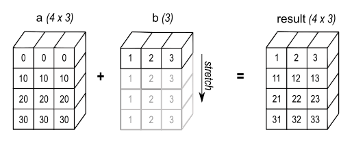
“Conceptually” matters. NumPy generally does not allocate a separate repeated copy of bias before doing the addition. It can reuse the original values through broadcast-aware indexing. The resulting shifted array, however, is a new array because it must hold newly computed values.
Broadcasting — NumPy v2.3 Manual
Read the NumPy manual’s explanation of broadcasting. It is the authoritative reference for the shape rules you will use constantly in numerical and deep-learning code.
In the opening “Broadcasting” section, read the motivation for broadcasting and vectorized operations. Then read the “General broadcasting rules” subsection. Study the compatibility rule, paying particular attention to the right-to-left comparison and the treatment of missing leading dimensions. In “Broadcastable arrays,” examine the examples involving shapes such as (5, 1), (1, 6), and (6,). Then find the later example where a (4, 3) array is combined with a length-3 vector, followed by the incompatible length-4 case. Finally, in “A practical example: vector quantization,” read the memory caution at the end of the section.
A shape ledger prevents most broadcasting mistakes
Before writing a broadcasted operation, write down the semantic role and shape of every operand. Treat this as part of the algorithm, not as debugging trivia.
Suppose scores contains examples, each with features:
scores.shape # (B, D)
To subtract each example’s own mean, the loop version might be:
def center_rows_loop(scores: np.ndarray) -> np.ndarray:
    result = np.empty_like(scores)

    for row_index in range(scores.shape[0]):
        row_mean = scores[row_index].mean()
        result[row_index] = scores[row_index] - row_mean

    return result
The vectorized version is:
row_means = scores.mean(axis=1, keepdims=True)
centered = scores - row_means
Its shape ledger is:
| Expression | Meaning | Shape |
|---|---|---|
scores |
batch of feature rows | |
scores.mean(axis=1, keepdims=True) |
one mean per row | |
scores - row_means |
subtract each row’s own mean |
keepdims=True is essential here. Without it:
scores.mean(axis=1).shape # (B,)
A shape of is aligned with the last axis of scores, not the first. NumPy would compare with , which usually raises an error. Worse, if , the expression could run while applying values along the wrong semantic axis.
When a reduction result must be combined back with the original array, ask:
Which axes were reduced, and should they remain as dimensions of size ?
For row-wise statistics, preserve the final feature axis with keepdims=True.
Creating a size-one axis explicitly
Sometimes your input has the right values but needs an explicit axis to express its intended role.
sample_scales = np.array([0.5, 1.0, 2.0])  # shape: (3,)

sample_scales = sample_scales[:, None]     # shape: (3, 1)
Now sample_scales can multiply a feature matrix of shape :
scaled_features = features * sample_scales
The shapes align as:
| Array | Shape |
|---|---|
features |
|
sample_scales |
|
| result |
None in an index inserts a new axis; np.newaxis is an equivalent spelling:
sample_scales[:, None]
sample_scales[:, np.newaxis]
This is the same structural idea used to create an outer operation:
row_values = np.array([10, 20, 30])     # (3,)
column_values = np.array([1, 2, 3, 4])  # (4,)

grid = row_values[:, None] + column_values[None, :]
print(grid.shape)
# (3, 4)
Here, one vector becomes and the other becomes , so both expand to .
An AI-relevant example: per-channel image normalization
Image preprocessing is full of broadcasting. Assume a channels-last batch of RGB images:
where for RGB. A loop-based channel normalization might look like this:
def normalize_images_loop(
    images: np.ndarray,
    mean: np.ndarray,
    std: np.ndarray,
) -> np.ndarray:
    result = np.empty_like(images, dtype=np.float32)

    batch_size, height, width, channels = images.shape

    for image_index in range(batch_size):
        for row_index in range(height):
            for column_index in range(width):
                for channel_index in range(channels):
                    result[
                        image_index,
                        row_index,
                        column_index,
                        channel_index,
                    ] = (
                        images[
                            image_index,
                            row_index,
                            column_index,
                            channel_index,
                        ]
                        - mean[channel_index]
                    ) / std[channel_index]

    return result
The broadcasted version is the mathematical statement itself:
normalized = (images - mean) / std
Its shapes are:
| Array | Shape | Semantic role |
|---|---|---|
images |
image batch | |
mean |
one mean per color channel | |
std |
one standard deviation per color channel | |
normalized |
normalized batch |
A vector with shape aligns with the last axis, precisely where channels live in this layout. NumPy conceptually views each statistic vector as .
images = np.random.default_rng(7).random(
    (8, 224, 224, 3),
    dtype=np.float32,
)

mean = np.array([0.485, 0.456, 0.406], dtype=np.float32)
std = np.array([0.229, 0.224, 0.225], dtype=np.float32)

normalized = (images - mean) / std
The layout is part of the contract. For channels-first data shaped , a vector of shape no longer aligns with the channel axis. You would reshape it to :
channel_mean = mean[None, :, None, None]
channel_std = std[None, :, None, None]

normalized_channels_first = (
    images_channels_first - channel_mean
) / channel_std
The reliable method is not memorizing special cases. Instead:
- Label the meaning of every axis.
- Identify the axis an operand should vary over.
- Insert size-one dimensions everywhere else.
- Check the resulting output shape before relying on the computation.
Refactor safely: preserve a baseline, then compare
Vectorized code is concise, but concise code can still express the wrong axis. During a refactor, retain the loop implementation briefly as a correctness oracle.
rng = np.random.default_rng(42)

features = rng.normal(size=(4, 6)).astype(np.float32)
bias = rng.normal(size=(6,)).astype(np.float32)

expected = add_bias_loop(features, bias)
actual = add_bias(features, bias)

np.testing.assert_allclose(actual, expected)
assert actual.shape == expected.shape
For floating-point calculations, use np.testing.assert_allclose rather than exact equality. Equivalent algebraic expressions can accumulate floating-point rounding differently, especially when reductions such as sum or mean are involved.
A practical refactoring sequence is:
- State the scalar equation, such as .
- Record the input and expected output shapes.
- Implement or retain a small loop-based baseline.
- Write the broadcasted expression.
- Compare values and shapes on representative small inputs.
- Only then measure performance on realistic input sizes.
The next lesson on pytest will turn this sort of one-time parity check into repeatable automated tests.
Broadcasting is powerful, not automatically free
Broadcasting avoids needless copies of the smaller operand, but it can still cause large outputs and large intermediate arrays.
For example, suppose you have feature vectors and code vectors, both with width :
points.shape     # (N, D)
codebook.shape   # (K, D)
A pairwise difference tensor can be written as:
differences = (
    points[:, None, :]
    - codebook[None, :, :]
)
The shape is:
For modest arrays this is clear and useful. It is also the basis of a straightforward nearest-code computation:
squared_distances = np.sum(
    (points[:, None, :] - codebook[None, :, :]) ** 2,
    axis=-1,
)
# shape: (N, K)
But the temporary difference array contains elements. With large batches, large codebooks, and high-dimensional embeddings, that can exhaust memory even if the final distance matrix is manageable.
The key distinction is:
- Broadcasting a small operand does not normally duplicate that operand in memory.
- The arithmetic operation may still materialize a large result.
- Chained expressions can create several temporary arrays.
When the broadcasted intermediate is too large, process the outer dimension in chunks or retain a deliberately chosen outer Python loop while vectorizing the inner numerical work. “No Python loops ever” is not the goal; the goal is to place loops at a granularity that is efficient, memory-safe, and readable.
Key takeaways
Broadcasting lets NumPy apply element-wise computations across compatible shapes without explicit element-by-element Python loops.
- Align shapes from the right.
- Dimensions are compatible when they are equal or one of them is .
- Missing leading dimensions behave as size-one dimensions.
- Use
None,np.newaxis, reshaping, orkeepdims=Trueto place a size-one dimension where the computation needs it. - Write down a shape ledger before vectorizing a loop.
- Keep a small loop baseline and compare results with
np.testing.assert_allcloseduring refactoring. - Broadcasting does not necessarily allocate repeated copies of a small input, but its outputs and intermediate arrays can still be very large.
- Element-wise operators such as
+,-,*, and/are not substitutes for matrix multiplication with@.
Next, you will make these numerical refactors dependable by writing parametrized pytest tests and reusable fixtures.