Analyzing Execution Plans for Slow Queries

A Quick Refresher: Reading Plans

Before we hunt for problems, let's quickly recall the golden rules for reading an execution plan, which you can find in the "Postgres Execution Plan" guide we looked at last time.

The core idea is that data flows from the most indented nodes (the leaves) up to the root. Our job is to follow that flow and find where the most time is being spent.

Red Flag #1: The Unnecessary Sequential Scan

One of the most common and impactful performance issues is the Sequential Scan (often shown as Seq Scan), also known as a full table scan.

A sequential scan means the database reads the entire table from disk, page by page, and checks every single row to see if it matches your WHERE clause.

• When is it OK? For small tables, or if your query needs to retrieve a large fraction of the table's rows.
• When is it a problem? For large tables where you only need a small, specific subset of rows. Imagine searching for one specific customer in a table with 10 million records by reading all 10 million records one by one.

This is almost always a symptom of a missing index on the column(s) in your WHERE clause.

How to Spot It

You'll see it plainly in the EXPLAIN output.

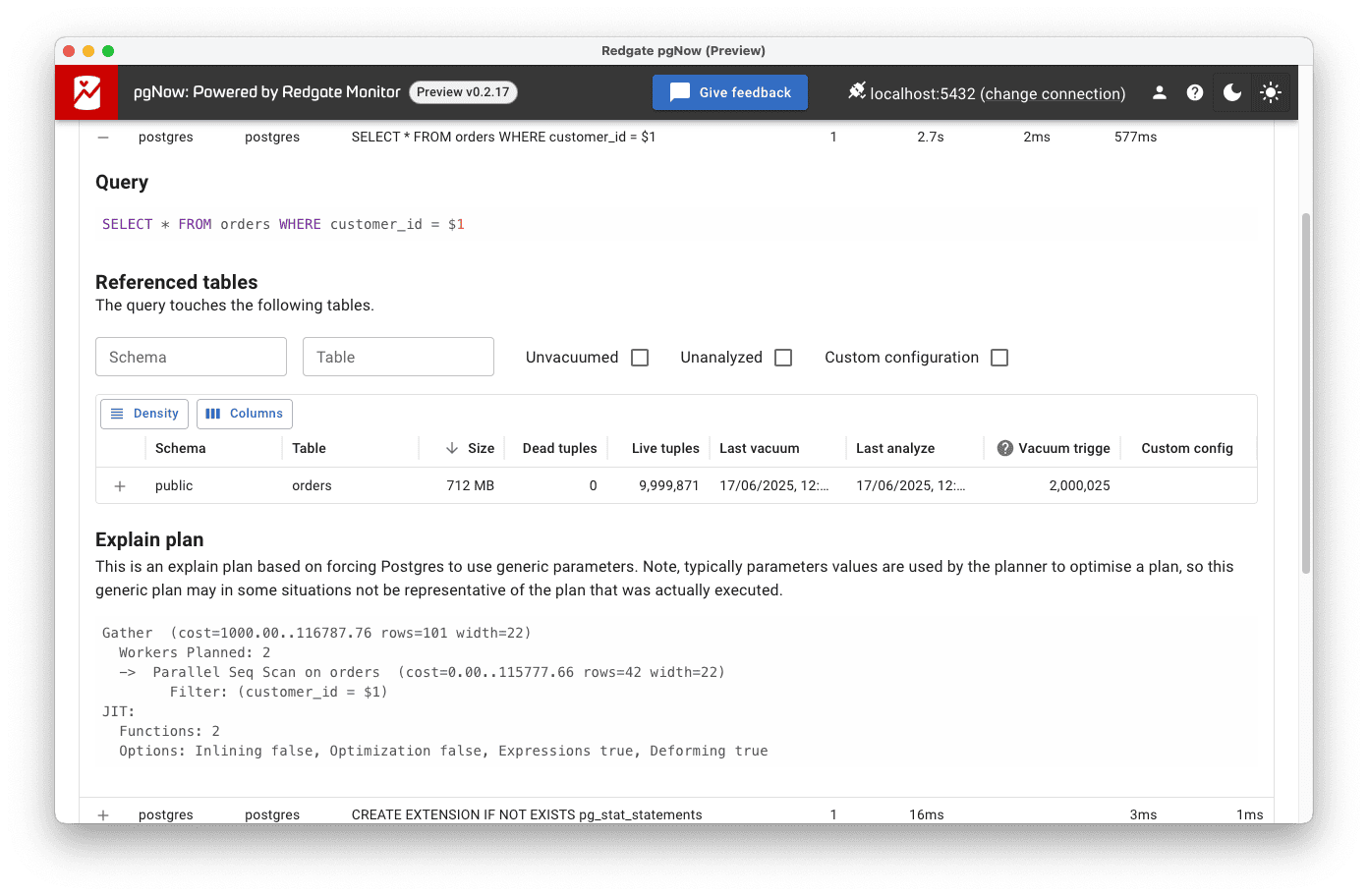
The solution is typically to add an index. Let's see a practical demonstration of identifying a sequential scan and the dramatic improvement an index provides.

As you saw, the difference is stark. The planner chose a Seq Scan for the volume_id query because it had no better option. It had to read every row. Once an index on id was used, it could go directly to the data it needed, transforming a slow operation into a nearly instantaneous one. This relates back to the random_page_cost we discussed; an index scan involves random disk access, but if it saves you from reading thousands of pages sequentially, it's a huge win.

Red Flag #2: The N+1 Query Problem

The N+1 problem is a notorious performance killer, especially when working with ORMs like Django's. Since you have experience with the Django REST Framework, you may have encountered this.

It happens when your code executes one query to retrieve a list of "parent" objects, and then executes N additional queries inside a loop to fetch a "child" object for each of the N parents.

Here is a classic Django example:

# authors is a list of N Author objects
authors = Author.objects.all() # Query 1

for author in authors: # Loop N times



    # This line triggers a new database query for each author
    books = author.books.all() # N additional queries!
    print(f"Author: {author.name}, Books: {list(books)}")

This pattern results in N+1 total queries to the database, which is extremely inefficient due to network latency and database overhead for each query.

While the N+1 problem often involves multiple distinct queries from the application, a very similar performance anti-pattern can occur within a single query. We can spot this signature in an EXPLAIN ANALYZE plan by looking for a Nested Loop join where the inner part of the loop is executed many times.

The key is the loops=N value.

Now, let's see how this appears in a plan. Imagine we have posts and comments tables and we run this query:

EXPLAIN ANALYZE
SELECT p.title, c.body
FROM posts p
JOIN comments c ON p.id = c.post_id
WHERE p.author_id = 123;

If we have an index on comments(post_id) but not on posts(author_id), the planner might produce a plan like this:

Nested Loop  (cost=1.00..5000.00 rows=2500 loops=1)
  ->  Seq Scan on posts p  (cost=0.00..1000.00 rows=500 loops=1)
        Filter: (author_id = 123)
  ->  Index Scan using comments_post_id_idx on comments c  (cost=1.00..8.00 rows=5 loops=500)
        Index Cond: (post_id = p.id)

Let's break down this plan to find the N+1 signature:

1. Seq Scan on posts: The database scans the entire posts table to find posts by author_id = 123. The actual rows (let's assume it's rows=500) tells us it found 500 posts. This is the "1" query.
2. Index Scan on comments: This is the inner part of the loop. Notice loops=500. This is the crucial red flag. It means the Index Scan on comments was executed 500 times—once for each post found in the step above.
3. The "N" Queries: This inner loop represents our "N" queries. Even though each index scan is fast (returning rows=5), the cumulative effect is significant. Total rows processed by the inner node are 5 rows * 500 loops = 2500 rows. The total time would be (time per loop) * 500.

The Solution:

• In the ORM, you'd use methods like Django's select_related or prefetch_related to tell the ORM to fetch the related objects more efficiently in a single, well-structured query (often a Hash Join).
• In raw SQL, the fix might be adding an index on posts(author_id) so the planner can choose a more efficient join strategy, or rewriting the query.

Other Common Causes of Slow Queries

While sequential scans and N+1 loops are the biggest offenders, here are a few other patterns to watch for.

1. Inefficient ORDER BY (Late Sorting)

If you ORDER BY a column that isn't indexed, the database must fetch all the results and then perform a costly Sort operation.

A key thing to watch for in EXPLAIN ANALYZE output for a sort is Sort Method: external merge on disk. This means the data to be sorted didn't fit in memory (work_mem) and the database had to use slow temporary files on disk. This is a major performance killer.

2. Inefficient Join Algorithms

The planner has several ways to join tables (e.g., Nested Loop, Hash Join, Merge Join). A poor choice can be disastrous.

• Nested Loop: Great when the outer table provides very few rows and the inner table is well-indexed. Terrible if the outer table returns many rows (the N+1 problem!).
• Hash Join: Generally good for joining large datasets. The planner builds an in-memory hash table on the smaller of the two tables and then streams the larger table through, probing the hash table for matches. Watch for Batches: 2 or more in EXPLAIN ANALYZE—this means the hash table didn't fit in memory and spilled to disk, slowing things down.
• Merge Join: Requires both inputs to be sorted on the join key. Very efficient if the data is already sorted (e.g., coming from an index scan), but can be slow if the database has to perform large, explicit sorts first.

3. Stale Statistics (Bad Estimates)

Always compare rows (estimated) with actual rows (from EXPLAIN ANALYZE). If there is a huge discrepancy (e.g., rows=10 but actual rows=500000), it means the planner's statistics are out of date. It made its decision based on bad information and likely chose a poor plan. The fix is simple: run ANALYZE your_table_name; to update the statistics, then re-analyze the query.

Conclusion

You've now moved from simply reading query plans to actively interpreting them for performance problems. By looking for these common anti-patterns, you can quickly diagnose the vast majority of slow SQL queries.

Key Takeaways:

• Seq Scan on a large table is a red flag. It often means you're missing an index on a WHERE or JOIN column.
• A Nested Loop with a high loops count is the signature of an N+1-style problem, where an inner operation is being wastefully repeated many times.
• A Sort node indicates the database had to manually sort results. If this is a bottleneck, consider adding an index on the ORDER BY column.
• Large differences between estimated and actual rows signal stale statistics. Run ANALYZE to fix this.

Preview of the Next Lesson

We have now reached the deepest part of the database layer in our journey. For the next module, we will move up the stack, away from the database and back towards the application server. The next lesson's objective is to build a minimal TCP server in Python using the socket module to accept and respond to connections.

This will take us back to the fundamentals of network programming, showing you what's happening at the operating system level before a tool like Gunicorn or even Django ever sees a request. This will provide the "root-level" understanding of server communication that you're looking for.