Understanding Database Join Algorithms

A High-Level Overview

At a conceptual level, these three algorithms approach the problem of matching rows from two tables in very different ways.

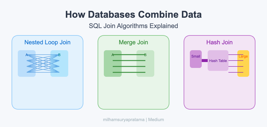
To build some initial intuition before we get into the technical details, let's start with a video that uses a simple card deck analogy to explain these concepts.

Now that you have a mental model for each algorithm, let's dive into the specifics of how they are implemented and when they are used.

The Cost of a Join

For the remainder of this lesson, our primary resources will be a detailed lecture and accompanying notes from Carnegie Mellon University's renowned database course. This aligns with your goal of going to the "deepest level as possible."

When we analyze these algorithms, we need a consistent way to measure their "cost." In a disk-based database, the most significant bottleneck is reading data from disk into memory (I/O). Therefore, our cost metric will be the number of disk I/Os. We'll ignore CPU costs for now, as I/O is orders of magnitude slower.

Let's establish our variables for the cost formulas:

• We are joining two tables, R (outer table) and S (inner table).
• M: The number of pages in table R.
• m: The number of tuples (rows) in table R.
• N: The number of pages in table S.
• n: The number of tuples (rows) in table S.
• B: The number of available pages in the buffer pool (the memory area the database uses).

1. Nested Loop Join

This is the most straightforward join algorithm. As the name implies, it's essentially two nested for loops.

Naive Nested Loop Join

The simplest implementation iterates through each tuple in the outer table R and, for each one, iterates through every single tuple in the inner table S to find matches.

for r in R:
  for s in S:
    if r.join_key == s.join_key:
      emit_match(r, s)

As you can imagine, this is incredibly inefficient if the tables are on disk. For every tuple in R, you might have to scan all N pages of S.

• Cost: $M+(m\times N)$

This is rarely used in practice unless the tables are tiny.

Block Nested Loop Join

A simple but effective optimization is to operate on blocks (pages) instead of individual tuples. For each page of the outer table R, you iterate through each page of the inner table S.

for r_page in R:
  for s_page in S:
    for r in r_page:
      for s in s_page:
        if r.join_key == s.join_key:
          emit_match(r, s)

The cost is reduced because we scan the inner table once per page of the outer table, not once per tuple.

• Cost: $M+(M\times N)$

We can improve this further by using the buffer pool to hold multiple pages of the outer table at once. If we use B-2 buffers for the outer table, the cost becomes:

• Cost: $M+(\lceil \frac{M}{B-2}\rceil \times N)$

Index Nested Loop Join

The most significant optimization occurs when we have an index on the join key of the inner table S. Instead of scanning S repeatedly, we can perform a highly efficient index lookup for each tuple in R.

for r in R:
  matches = index_on_S.lookup(r.join_key)
  for s in matches:
    emit_match(r, s)

The cost now depends on the cost of the index lookup, C.

• Cost: $M+(m\times C)$

If the index is highly selective, this can be extremely fast. This is why having proper indexes on foreign keys is crucial for performance.

2. Sort-Merge Join

The Sort-Merge Join tackles the problem differently. It has two distinct phases:

1. Sort Phase: Sort both tables, R and S, on the join key. If the data is large, the database will use an external merge sort algorithm (like the one we discussed in a previous module context).
2. Merge Phase: With both tables sorted, the database can merge them in a single, linear pass. It uses two cursors, one for each table, and advances them in lockstep. If the keys match, it emits the joined rows. If not, it advances the cursor pointing to the smaller key.

This algorithm is particularly effective if:

• One or both tables are already sorted on the join key (e.g., due to a clustered index).
• The final query result needs to be sorted by the join key anyway (ORDER BY).

A complication arises with duplicate keys. If a key in R matches multiple keys in S, the cursor for S must backtrack to the start of the matching block for each duplicate in R.

• Cost: Sort Cost(R) + Sort Cost(S) + Merge Cost(R, S)
  • The sort cost is the cost of the external sort for each table.
  • The merge cost (in the best case with few duplicates) is simply $M+N$, as each page is scanned only once.

3. Hash Join

The Hash Join is often the fastest algorithm for large, unsorted equi-joins (joins using the = operator). Like the Sort-Merge Join, it has two phases:

1. Build Phase: The database scans the smaller table (let's say R) and builds a hash table in memory, using the join key as the hash key.
2. Probe Phase: The database then scans the larger table (S), one tuple at a time. For each tuple s, it hashes its join key and probes the hash table to find a match from R.

This is extremely efficient because a hash table lookup is a very fast operation.

But what if the smaller table R is too large to fit in memory? This is where the Partitioned Hash Join (also known as the Grace Hash Join) comes in.

1. Partitioning Phase (Build): The database scans both tables, R and S. It applies a hash function (h1) to the join key of each tuple and writes the tuples out to separate partitions on disk. Because the same hash function is used, all matching tuples from R and S are guaranteed to end up in the same pair of partitions.
2. Probing Phase (Join): For each pair of partitions (e.g., R_i and S_i), the database loads them into memory one by one. Since the partitions are small enough, it can now perform an in-memory Hash Join on them: build a hash table on R_i and probe it with S_i.

If a partition is still too large to fit in memory, the database can recursively apply the partitioning process with a different hash function (h2).

• Cost (Partitioned Hash Join): 3 * (M + N)
  • Read R and S to create partitions (M+N).
  • Write the partitions of R and S to disk (M+N).
  • Read the partitions back in to perform the joins (M+N).

The Query Optimizer's Choice

So, which algorithm does the database choose? This critical decision is made by the query optimizer. Before executing a query, the optimizer generates multiple possible execution plans, each using different join algorithms and join orders.

It uses an internal cost model, factoring in:

• Table statistics: Number of rows, number of pages, data distribution (cardinality).
• Available indexes: An index on a join key makes an Index Nested Loop Join a very strong candidate.
• Query predicates: WHERE clauses, ORDER BY clauses.
• System resources: Available memory for hash tables or sorting.

The optimizer estimates the I/O cost for each plan and picks the one it predicts will be the cheapest. This is why EXPLAIN plans can change if your data size or distribution changes, or if you add/remove an index.

Conclusion

You now have a solid, deep understanding of how databases execute one of their most fundamental operations. This knowledge moves you from being a user of the database to an informed developer who can reason about its internal behavior.

Key Takeaways:

• Nested Loop Join: Simple but often slow. It becomes highly effective (Index Nested Loop Join) when an index is available on the inner table's join key. It's great for joining a small number of rows to a large table via an index.
• Sort-Merge Join: Shines when one or both inputs are already sorted. It consists of a Sort phase and a Merge phase and produces a sorted output, which can be an added benefit.
• Hash Join: Generally the most efficient for large, unsorted equi-joins. It uses a Build phase and a Probe phase. The Partitioned Hash Join variant allows it to handle data that is much larger than available memory.
• The Query Optimizer: This is the "brain" that chooses the best algorithm by estimating the cost of various execution plans based on table statistics and available indexes.

Preview of the Next Lesson

We've covered how the database executes queries. But a backend server is rarely serving just one user at a time. What happens when hundreds of requests are trying to read and write to the same tables simultaneously?

In the next lesson, we will explore database concurrency. We'll learn about ACID properties, transactions, and the different transaction isolation levels (e.g., Read Committed, Serializable) that databases use to guarantee data consistency without bringing the whole system to a halt.