PyTorch Training Loop: A Complete Walkthrough

The Anatomy of a Training Loop

At its heart, training a neural network is a cycle of guessing, checking, and correcting. We repeat this cycle over and over until the model's "guesses" are as accurate as possible. One full pass through the entire dataset is called an epoch. Within each epoch, we process the data in small groups called batches. The training loop operates on these batches.

The entire process can be broken down into five fundamental steps, which are beautifully illustrated in the diagram below.

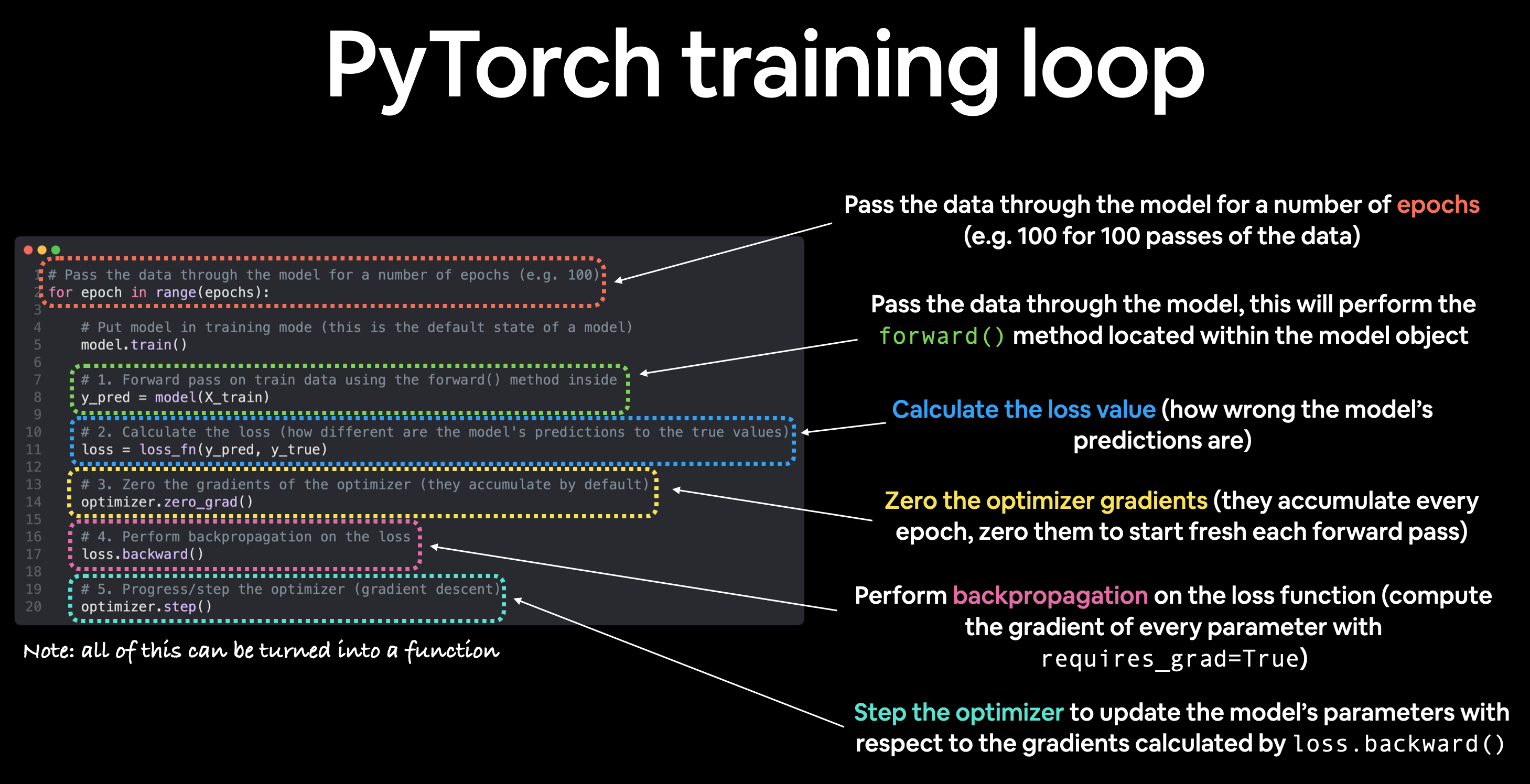
Let's break down what each of these steps means:

1. Forward Pass: We pass a batch of input data through the model to get its predictions.
2. Calculate Loss: We compare the model's predictions to the true labels using a loss function. This function outputs a single number (the "loss") that quantifies how wrong the model was.
3. Zero Gradients: We reset the gradients of all model parameters. This is a crucial housekeeping step to prevent gradients from previous batches from accumulating.
4. Backpropagation: We compute the gradient of the loss with respect to each model parameter. This is where PyTorch's autograd engine does its magic, figuring out how much each parameter contributed to the overall error. This is conceptually the "blame assignment" step.
5. Step the Optimizer: We use an optimizer to update the model's parameters in the direction that will reduce the loss.

To perform these steps, we need two key components that we haven't discussed yet: a loss function and an optimizer.

The Learning Components: Loss Function and Optimizer

Before we can write the loop, we need to define how the model measures its error and how it should update itself.

• A Loss Function (or criterion) measures the discrepancy between the model's prediction and the ground truth. For a classification task like yours (e.g., classifying meal quality as 'Good', 'Adequate', or 'Poor'), the most common choice is nn.CrossEntropyLoss. It's particularly well-suited for multi-class problems.

• An Optimizer is an algorithm that adjusts the model's parameters (weights and biases) based on the computed gradients. A very popular and effective all-around optimizer is Adam. It requires the model's parameters and a learning_rate, which controls the size of the update steps.

This resource from Microsoft Learn provides a concise explanation of these two components.

The Three-Line Mantra of Learning

The core of the learning process—steps 3, 4, and 5—can be distilled into a simple, powerful three-line pattern that you will use constantly in PyTorch. The video below offers a superb conceptual explanation of backpropagation and introduces this "three-line mantra."

Implementing the Full Loop

Now, let's assemble everything into a complete training loop. We'll have an outer loop for the epochs and an inner loop that iterates through the batches provided by a DataLoader.

The following official PyTorch tutorial provides a well-structured example inside a train_one_epoch function.

To make this concrete, here is a complete, commented Python script that ties together all the concepts from this module. It defines a simple model, sets up a dummy DataLoader, and runs the full training loop.

import torch
import torch.nn as nn
from torch.utils.data import TensorDataset, DataLoader




# --- 1. Setup and Hyperparameters ---
# Device configuration (from a previous lesson)
device = torch.device("cuda" if torch.cuda.is_available() else "cpu")
print(f"Using device: {device}")




# Hyperparameters
NUM_EPOCHS = 5
BATCH_SIZE = 16
LEARNING_RATE = 0.001




# --- 2. Create a Dummy Dataset and DataLoader ---
# This simulates your actual data pipeline (from the previous lesson)
# Let's create a simple regression problem: y = 2*x1 + 3*x2 + noise
X = torch.randn(100, 2)  # 100 samples, 2 features
y = 2 * X[:, 0] + 3 * X[:, 1] + torch.randn(100) * 0.1
y = y.view(-1, 1) # Reshape y to be a column vector

dataset = TensorDataset(X, y)
data_loader = DataLoader(dataset=dataset, batch_size=BATCH_SIZE, shuffle=True)




# --- 3. Define the Model, Loss, and Optimizer ---
# Model (from a previous lesson)
model = nn.Sequential(
    nn.Linear(2, 1) # Simple linear model with 2 inputs and 1 output
).to(device)




# Loss Function
loss_fn = nn.MSELoss() # Mean Squared Error for this regression task




# Optimizer
optimizer = torch.optim.Adam(model.parameters(), lr=LEARNING_RATE)




# --- 4. The Training Loop ---
for epoch in range(NUM_EPOCHS):



    # Set the model to training mode
    model.train() 
    
    for i, (inputs, labels) in enumerate(data_loader):



        # Move tensors to the configured device
        inputs = inputs.to(device)
        labels = labels.to(device)
        



        # STEP 1: Forward pass
        outputs = model(inputs)
        



        # STEP 2: Calculate the loss
        loss = loss_fn(outputs, labels)
        



        # STEP 3: Zero the gradients
        optimizer.zero_grad()
        



        # STEP 4: Backward pass (backpropagation)
        loss.backward()
        



        # STEP 5: Update the weights
        optimizer.step()
        



    # Print progress every epoch
    print(f'Epoch [{epoch+1}/{NUM_EPOCHS}], Loss: {loss.item():.4f}')

print("Training finished!")



# After training, we can inspect the learned parameters
# They should be close to our true values of [2, 3] for weight and ~0 for bias.
for name, param in model.named_parameters():
    if param.requires_grad:
        print(name, param.data)

Training vs. Evaluation Mode

You might have noticed the model.train() line in the code above. This is important because some layers, like nn.Dropout or nn.BatchNorm2d, behave differently during training and evaluation.

• model.train(): Puts the model in "training mode". This enables behaviors like dropout.
• model.eval(): Puts the model in "evaluation mode". This disables dropout and uses running statistics for batch normalization, ensuring deterministic outputs.

When you are testing your model or using it for inference, you should always call model.eval() first. Furthermore, during evaluation, there's no need to compute gradients. You can disable gradient computation using the torch.no_grad() context manager, which saves memory and speeds up computations.

Here is how you would typically structure an evaluation loop:

# Assume validation_loader is a DataLoader for your test/validation set
model.eval() # Set the model to evaluation mode
with torch.no_grad(): # Disable gradient calculation
    total_loss = 0
    for inputs, labels in validation_loader:
        inputs = inputs.to(device)
        labels = labels.to(device)
        
        outputs = model(inputs)
        loss = loss_fn(outputs, labels)
        total_loss += loss.item()

avg_val_loss = total_loss / len(validation_loader)
print(f'Average Validation Loss: {avg_val_loss:.4f}')

Conclusion

Congratulations on completing the PyTorch Fundamentals module! You now possess the complete toolkit to build, train, and evaluate neural networks. From tensors to data loaders to the training loop itself, you have a solid foundation to tackle your multimodal project.

Let's recap the key takeaways from this lesson:

• The training loop is a five-step cycle: forward pass, loss calculation, zeroing gradients, backpropagation, and optimizer step.
• The loss function (nn.CrossEntropyLoss for classification) quantifies model error.
• The optimizer (torch.optim.Adam) updates model parameters to minimize the loss.
• The learning process is driven by the "three-line mantra": optimizer.zero_grad(), loss.backward(), and optimizer.step().
• It's crucial to switch between training and evaluation modes using model.train() and model.eval(), and to use with torch.no_grad() during evaluation.

With these fundamentals established, we are ready to move from theory to practice. In the next module, we will begin the first real step of your project: data acquisition. Your next lesson will guide you through using the PRAW library to scrape the text complaints and associated metadata from Reddit, which will become the foundation for your text-based classification model.