GPU-Accelerated CNN Fine-Tuning for Meal Image Analysis

1. The Anatomy of a Training Loop

Training a neural network in PyTorch is an active process that you control with a script. At its heart, a training loop iterates over your dataset multiple times. Each full pass over the dataset is called an epoch. Within each epoch, the data is processed in small batches, as provided by your DataLoader.

Critically, each epoch is typically split into two distinct phases:

• Training Phase: The model processes training data, and its weights are updated to minimize error. We use model.train() to put the model in this mode.
• Validation Phase: The model processes a separate set of unseen validation data. Its performance is measured, but its weights are not updated. This is crucial for assessing how well the model generalizes and for detecting overfitting. We use model.eval() to switch to this mode.

The switch between train() and eval() modes is important because certain layers, like Dropout and batch normalization, behave differently during training and inference.

2. The Core Machinery: Optimizer and Loss Function

Before we can write the loop, we need two key components:

• Loss Function (Criterion): This function measures how far the model's prediction is from the actual label. For a multi-class classification problem like yours (Good, Adequate, Poor), the standard choice is Cross-Entropy Loss (nn.CrossEntropyLoss). It combines the model's output scores (logits) with the true class label into a single value representing the error.
• Optimizer: This is the algorithm that updates the model's weights to reduce the loss. It takes the gradients computed during backpropagation and uses them to take a "step" in the right direction. A common and effective choice is the Adam optimizer (torch.optim.Adam). You'll also need to set a learning rate, a hyperparameter that controls the size of the update step.

In the previous lesson, we froze the convolutional base, so only the new fc layer has parameters that require gradients. The optimizer will only update these parameters.

# Assume 'model' is the ResNet-50 we prepared in the last lesson
# and 'device' is set to "cuda"




# Loss function
criterion = nn.CrossEntropyLoss()




# Optimizer
# We pass only the parameters of the final layer to the optimizer
optimizer = torch.optim.Adam(model.fc.parameters(), lr=0.001)

3. Implementing the Full Training Loop

Now we can assemble the full loop. The following steps happen for each batch in the training phase:

1. Move Data to GPU: Transfer the batch of images and their labels to the GPU.
2. Zero Gradients: Clear any gradients from the previous step using optimizer.zero_grad().
3. Forward Pass: Pass the images through the model to get predictions: outputs = model(inputs).
4. Calculate Loss: Compute the error between the predictions and true labels: loss = criterion(outputs, labels).
5. Backward Pass: Calculate the gradients of the loss with respect to the model's weights: loss.backward().
6. Update Weights: The optimizer updates the weights based on the computed gradients: optimizer.step().

The official PyTorch tutorial on transfer learning contains an excellent function, train_model, that encapsulates this entire logic. It's a robust template that you can adapt for your project.

The tutorial you just reviewed is the canonical way to structure a training loop in PyTorch. The blog post from Leonie Monigatti offers a slightly different, but equally valid, way to organize the code by separating the training and validation logic into two distinct functions, train_one_epoch and validate_one_epoch. This can sometimes make the code even easier to read.

4. Feature Extraction vs. Fine-Tuning

So far, we have been implementing the feature extraction strategy: we froze the convolutional base and are only training the new classification head. This is fast and works well for small datasets.

Fine-tuning, in the stricter sense, involves un-freezing the entire model (or the last few layers of it) and continuing to train all of them, but with a very low learning rate. This allows the pretrained feature detectors to adapt slightly to the specifics of your meal images, which can lead to better performance.

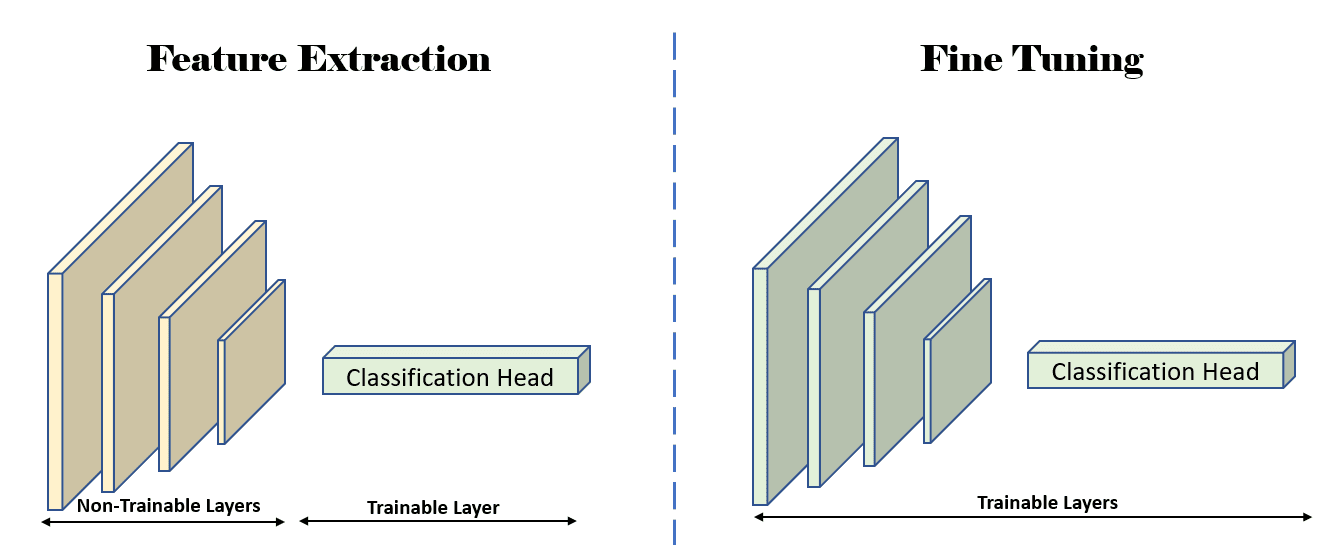
To implement fine-tuning, you would simply pass all the model's parameters to the optimizer, instead of just model.fc.parameters().

# For fine-tuning, you would un-freeze the layers and optimize all parameters
# Note: You would typically use a much smaller learning rate (e.g., 1e-5)
# for the pretrained layers compared to the new classifier head.
# For simplicity here, we use one learning rate for all.




# Un-freeze all parameters
for param in model.parameters():
    param.requires_grad = True




# Optimizer now takes all model parameters
optimizer = torch.optim.Adam(model.parameters(), lr=0.0001)

For your first baseline model, sticking with the feature extraction approach is recommended as it's faster and less prone to overfitting with a small dataset. However, knowing how to switch to full fine-tuning is an important skill for later experiments.

The following video provides a practical, step-by-step walkthrough of this whole process, from setting up the data to running the training loop.

Conclusion

You now have a complete roadmap for training your first image classification model. By combining the pretrained model architecture from our last lesson with the training loop discussed today, you can build and train a powerful baseline for your project.

Here are the key takeaways from this lesson:

• The training process is managed by a training loop that iterates over your data in epochs and batches.
• Each epoch includes a training phase (to update weights) and a validation phase (to measure generalization).
• The loss function (nn.CrossEntropyLoss) quantifies model error, and the optimizer (torch.optim.Adam) uses this error to update model weights.
• Fine-tuning can refer to the general process of adapting a model, but more specifically to un-freezing pretrained layers and training them at a low learning rate.
• For effective GPU acceleration, both the model and the data tensors for each batch must be moved to the GPU using .to(device).

You have trained your model, but how good is it really? An overall accuracy score can be deceiving. In our next lesson, we will explore a more sophisticated set of tools for evaluating your image classifier's performance, including precision, recall, F1-score, and the confusion matrix, to gain a deeper understanding of its strengths and weaknesses.