Welcome to Module 8. In the last few lessons, we've focused intensely on building and validating the predictive core of your project. You successfully fine-tuned models for image and text data and then fused them into a more powerful multimodal system, proving its superior performance. Now, we shift our focus from what the violations are to where they are happening.
This lesson marks the beginning of your journey into geospatial analysis. Our goal is to load and manipulate geographic data (e.g., district shapefiles) using GeoPandas. This is the foundational skill you'll need to create the hotspot maps and regional analyses that are central to your project's sixth week. By the end of this session, you'll be able to read geographic files, understand their structure, and perform basic operations, setting the stage for visualizing your model's predictions on a map.
What is GeoPandas?
GeoPandas is a powerful open-source library that extends the datatypes used by pandas to allow spatial operations on geometric types. If you think of pandas as your tool for wrangling tabular data (rows and columns), GeoPandas is your tool for wrangling geographic data—data that has a physical location on Earth.
Since you're proficient with Python and its data science ecosystem, you'll find GeoPandas feels very familiar. It's built on top of several key libraries:
- Pandas: Provides the
DataFramestructure that GeoPandas extends. - Shapely: Used for handling and manipulating geometric objects (like points, lines, and polygons).
- Fiona: Handles reading and writing data from various geospatial file formats.
- pyproj: Manages coordinate reference systems and projections.
The following short video gives a concise overview of how these pieces fit together.
This video from the Geospatial Programming channel explains what GeoPandas is and the libraries it is built upon.
Watch the first 30 seconds of the video, from the introduction, to understand how GeoPandas leverages other libraries to add geospatial capabilities to Python.
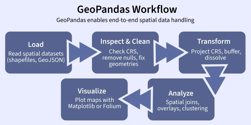
The typical end-to-end process of working with spatial data in GeoPandas can be summarized in a simple workflow, from loading data to visualizing it.
Reading and Inspecting Geographic Data
The first step in any geospatial task is loading your data. Geographic vector data comes in many formats, but the most common one you'll encounter is the Shapefile (.shp). It's important to know that a shapefile isn't a single file, but a collection of files that work together. Typically, you'll see at least three:
.shp: Contains the feature geometry (the shapes themselves)..shx: An index file for the geometries..dbf: A database file that stores the attribute information for each feature (like a district's name or population)..prj: Contains the coordinate reference system information.
GeoPandas simplifies this by letting you point to the .shp file, and it automatically finds and uses the associated files. The primary function for this is gpd.read_file().
GeoPandas Basics: Maps, Projections, and Spatial Joins
This article from Real Python provides a clear introduction to loading data and understanding the structure of a GeoDataFrame.
Read the sections Reading in Data and the subsequent two paragraphs. Focus on how gpd.read_file() is used and the description of the GeoDataFrame and GeoSeries objects, particularly the special geometry column.
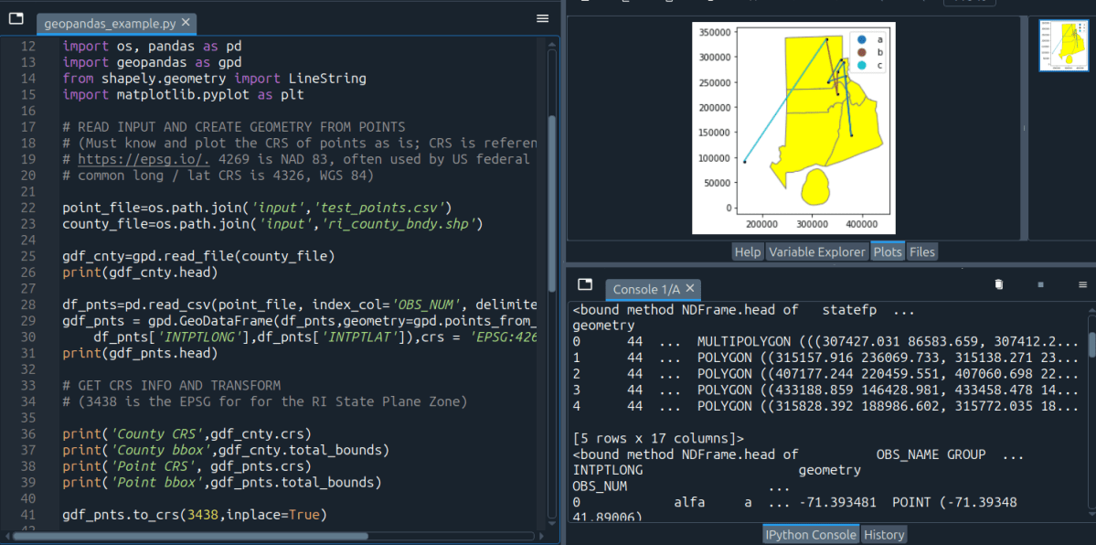
As you just read, the gpd.read_file() function returns a GeoDataFrame. This object is the heart of GeoPandas. It is, for all practical purposes, a pandas DataFrame but with a special column, typically named geometry, that stores the geometric information. All the pandas functions you already know—head(), info(), filtering with boolean masks—work exactly as you'd expect.
The Anatomy of a GeoDataFrame
Let's dig a little deeper into the geometry column. This column doesn't just store numbers or text; it holds Shapely objects. These can be Point, LineString, or Polygon objects (or their "multi" counterparts like MultiPolygon). Because these are rich geometric objects, you can directly perform spatial calculations on them.
A common operation is calculating the area of polygons. A GeoDataFrame has a .area attribute that computes the area for each geometry in the geometry column and returns a pandas Series.
Introduction to Geopandas — Intro to Python GIS CSC ...
The "Automating GIS Processes" course documentation provides a practical, step-by-step guide to working with GeoDataFrames.
First, read the section Reading a Shapefile to reinforce how data is loaded. Then, jump to the section Geometries in Geopandas and continue reading until the end of that section, where it calculates the mean area. Pay close attention to how the geometry column is accessed and how the .area attribute is used to perform a vectorized calculation across all polygons.
Basic Visualization with .plot()
One of the most satisfying parts of working with GeoPandas is how easy it is to create a map. A GeoDataFrame has a .plot() method that, instead of creating a chart, generates a map of the geometries. This is incredibly useful for a quick visual check to ensure your data loaded correctly.
The following video provides an excellent walkthrough of reading a shapefile and creating basic plots, including how to customize their appearance.
An Absolute Beginner's Guide to Python GeoPandas
This video from GeoDelta Labs gives a beginner-friendly, hands-on demonstration of loading and plotting data with GeoPandas.
Watch from loading a shapefile to see how gpd.read_file() works in practice and how the resulting GeoDataFrame is inspected. Then, continue watching from the plotting section. Focus on how the .plot() method is used and how you can layer multiple datasets and customize colors, which will be essential for creating your final project maps.
A Crucial Concept: Coordinate Reference Systems (CRS)
You might have noticed the coordinates in the examples look like large numbers, not the familiar latitude and longitude. This is because the data is in a specific Coordinate Reference System (CRS). A CRS is a framework used to define how the 3D surface of the Earth is projected onto a 2D map.
There are two main types of CRS:
- Geographic CRS: Uses latitude and longitude on a spherical or ellipsoidal model of the Earth (e.g., WGS84, EPSG:4326). Units are in degrees.
- Projected CRS: Flattens the Earth's surface onto a 2D plane (e.g., UTM zones). This introduces distortion but allows for measurements in meters or feet, which is necessary for accurate area or distance calculations.
For your project, you must ensure all your geographic datasets are in the same CRS before you can combine or analyze them together. GeoPandas makes this easy.
- You can check a
GeoDataFrame's CRS with the.crsattribute. - You can change (reproject) it to a new CRS with the
.to_crs()method.
The same video provides a very clear explanation of why this matters and how to do it.
An Absolute Beginner's Guide to Python GeoPandas
This segment of the video explains what a CRS is and demonstrates how to check and reproject it in GeoPandas.
Watch the segment on projections. The instructor clearly explains how to check the CRS using .crs and transform it using .to_crs(), showing the visual difference between a geographic and a projected CRS.
Creating and Saving Geographic Data
Finally, after loading and manipulating your data, you'll need to save your results. Just as you can read files with read_file(), you can write them with to_file(). This allows you to save your modified GeoDataFrame as a new shapefile, GeoJSON, or other format.
Furthermore, a key task in your project will be to create geographic data from your model's outputs. For example, you will calculate a "violation score" for each district. This data will exist in a regular pandas DataFrame. To map it, you will need to create a GeoDataFrame by combining your tabular data with geometric shapes.
The process is straightforward: you can construct a GeoDataFrame from a pandas DataFrame by specifying which column contains the geometry objects.
Introduction to Geopandas — Intro to Python GIS CSC ...
This resource also covers the full circle of creating and writing data.
First, read the short section Writing a Shapefile to see how to_file() works. Then, carefully read the entire section Creating geometries into a GeoDataFrame. This is a critical skill. It walks you through creating a GeoDataFrame from scratch, adding attributes, setting the CRS, and finally saving it. This is the exact workflow you'll use to combine your model's violation scores with district boundaries.
Conclusion
In this lesson, you've taken your first steps into the world of geospatial analysis with Python. You've learned how GeoPandas extends the familiar pandas DataFrame to handle geographic data, making complex spatial tasks accessible through a clean, programmatic interface.
Here are the key takeaways:
- GeoDataFrame: The core data structure in GeoPandas, which is a pandas DataFrame with a special
geometrycolumn. - Reading and Writing: You can easily load geographic files like shapefiles with
gpd.read_file()and save them with.to_file(). - Manipulation and Plotting: You can manipulate
GeoDataFramesjust like you would aDataFrameand create quick visualizations with the.plot()method. - Coordinate Reference Systems (CRS): Understanding and managing CRS with
.crsand.to_crs()is essential for accurate analysis and for combining different datasets.
You now have the foundational skills to handle the "geo" part of your project's geospatial component. Your next step will be to merge your model's prediction data with these geographic dataframes. In our next lesson, we will focus on exactly that: performing attribute and spatial joins to link your violation data to specific districts, preparing it for visualization.