Scaled Dot-Product Attention Calculation

Introduction

In our last lesson, we focused on the initial step of the attention mechanism: calculating raw relevance scores by taking the dot product of Query and Key vectors. This yielded an $N \times N$ matrix, $S = Q K^{T}$ , where each entry $S_{ij}$ represents the raw, unbounded relevance of token $j$ to token $i$ . While these scores capture the fundamental relationships, they are not yet in a usable form to directly manipulate the token embeddings.

This lesson completes the picture by walking through the rest of the scaled dot-product attention formula. Our goal is to transform these raw scores into a normalized probability distribution and then use this distribution to create new, context-aware embeddings for each token. We will follow this celebrated formula as our guide:

Attention (Q, K, V) = softmax (\frac{Q K ^{T}}{d _{k}}) V

We will dissect this computation step-by-step: scaling the scores, applying the softmax function to get attention weights, and finally, multiplying by the Value matrix to produce the mechanism's output.

The Full Computation: From Raw Scores to Context Vectors

The entire process can be broken down into four distinct steps. We've already covered the first (computing $Q K^{T}$ ). Now let's proceed with the remaining three.

A great resource that walks through this entire sequence is the article "Demystifying Scaled Dot-Product Attention" from PyML Studio. We will use it as our primary guide, supplemented by video explanations.

First, let's get a high-level overview of the entire process from start to finish.

Attention is all you need (Transformer) - Model explanation (including math), Inference and Training

The video "Attention is all you need" by Umar Jamil provides a concise, math-centric walkthrough of the self-attention calculation.

Watch the segment from this walkthrough. The narrator explains how the input matrix (which serves as Q, K, and V) is processed through the formula. Focus on the sequence of operations: the matrix multiplication of Q and K transpose, the division (scaling), the application of softmax, and the final multiplication by V. Also, note the dimensions of the matrices at each stage.

Now, let's break down each of these steps in more detail.

Step 1: Scaling the Compatibility Matrix

Having computed the compatibility matrix $Q K^{T}$ , the first operation applied is scaling. We divide every element in the matrix by $d_{k}$ , where $d_{k}$ is the dimension of the key (and query) vectors.

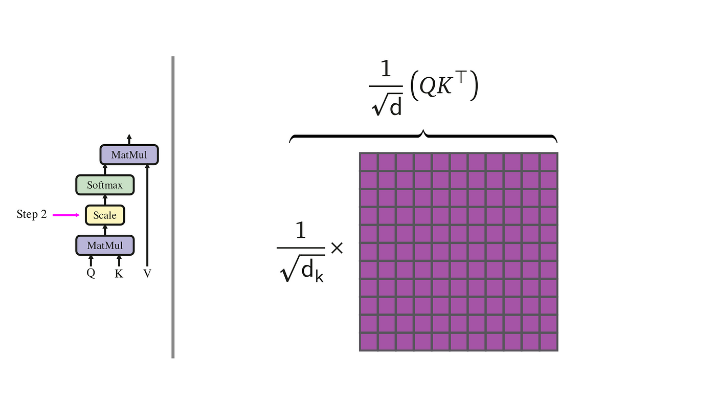
The compatibility matrix, representing the dot products of Q and K^T, is scaled by dividing each element by the square root of the key vector dimension, d_k.

This step is crucial for stabilizing the training process, particularly when dealing with large vector dimensions. The scaling prevents the dot product values from becoming too large, which would push the softmax function into regions with very small gradients, hindering learning. We will dedicate the next lesson to a deeper mathematical justification for why this specific scaling factor is used. For now, we will focus on the computation itself.

Demystifying Scaled Dot-Product Attention - PyML Studio

The PyML Studio article provides a clear explanation of this scaling step, complete with a PyTorch code example and visualizations.

Please read the section titled "Step 2: Scaling." Pay attention to the simple implementation and the author's note on why unscaled attention underperforms for large dimensions. The visualization comparing heatmaps before and after scaling is particularly illustrative.

Step 2: Normalization with Softmax

After scaling, we have a matrix of scores that are better behaved, but they are still just arbitrary real numbers. To use them as weights in a weighted average, we need to convert them into a probability distribution. This is achieved using the softmax function.

You'll recall from your deep learning fundamentals that the softmax function, given by $σ (z)_{i} = \frac{e ^{z_{i}}}{\sum _{j} e ^{z_{j}}}$ , transforms a vector of arbitrary real numbers into a vector of values between 0 and 1 that sum to 1.

In the attention mechanism, we apply softmax to each row of the scaled compatibility matrix independently. The $i$ -th row of the matrix contains the relevance scores of every token in the sequence with respect to the $i$ -th token's query. Applying softmax to this row converts these scores into a set of attention weights, $a_{i}$ , where the weight $a_{ij}$ represents how much attention token $i$ should pay to token $j$ , and $\sum_{j} a_{ij} = 1$ .

The softmax function is applied to each row of the scaled compatibility matrix, converting the scores into normalized attention weights that sum to 1 for each row.

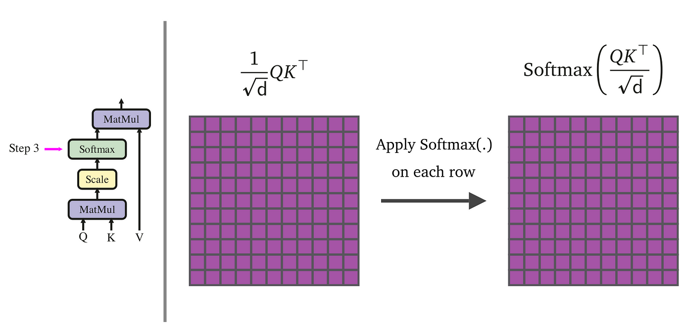
The resulting matrix is the attention matrix, which encapsulates the final, normalized weights.

Demystifying Scaled Dot-Product Attention - PyML Studio

This next section of the article details the application of the softmax function.

Read the section "Step 3: Softmax Normalization." This part recaps the properties of the softmax function and shows how it's applied in PyTorch to produce the final attention weights matrix.

Step 3: Producing the Output via Weighted Sum

We now have our attention weights matrix, $A = softmax (\frac{Q K ^{T}}{d _{k}})$ . The final step is to use these weights to create the new, context-aware embeddings. This is where the Value matrix, V, comes into play.

The output of the attention mechanism is computed by multiplying the attention matrix $A$ by the Value matrix $V$ :

Output = A \cdot V

Let's analyze this matrix multiplication more closely. The output embedding for a single token $i$ , which is the $i$ -th row of the output matrix, is calculated as:

output_{i} = j = 1 \sum N a_{ij} v_{j}

This is a weighted sum of all value vectors in the sequence. The weights are precisely the attention scores we just computed. In essence, for each token, we are creating a new embedding by blending the "content" (the value vectors) of all tokens in the sequence, with the amount of blend determined by the relevance of each token. A token with a high attention weight $a_{ij}$ will contribute significantly its value vector $v_{j}$ to the new representation of token $i$ .

This final multiplication is the step where information is actually aggregated and moved between tokens, producing a set of output vectors that are no longer isolated but are now enriched with context.

Attention in transformers, step-by-step | Deep Learning Chapter 6

The 3Blue1Brown video, "Attention in transformers, step-by-step," offers a superb visual explanation of this final weighted sum.

Please watch the segment from this section on the weighted sum. The animation clearly shows how the attention weights for a specific column (representing the token being updated) are used to scale the value vectors from all other tokens, which are then summed up to create the final output embedding.

Finally, let's complete our reading of the PyML Studio article to see this last step in practice.

Demystifying Scaled Dot-Product Attention - PyML Studio

The final part of the article covers the multiplication with the Value matrix.

Read the short section titled "Step 4: Generating the Context Vectors." It shows the final matrix multiplication and confirms that the output matrix has the expected dimensions, matching the dimensionality of the value vectors.

Conclusion

In this lesson, we have assembled the complete scaled dot-product attention mechanism, starting from the raw query-key dot products and ending with a set of contextually enriched output vectors.

Here are the key computational steps we've established:

Compute Raw Scores: Calculate the dot product of all query-key pairs, typically via the matrix multiplication $Q K^{T}$ .
Scale: Divide all raw scores by $d_{k}$ , the square root of the key vector dimension, to stabilize gradients during training.
Normalize: Apply the softmax function to each row of the scaled score matrix. This converts the scores into a probability distribution, yielding the final attention weights matrix $A$ .
Aggregate Values: Compute the final output by multiplying the attention weights matrix $A$ by the Value matrix $V$ . The resulting output is a matrix where each row is a new embedding for the corresponding input token, created as a weighted sum of all value vectors in the sequence.

You now understand the complete data flow through a scaled dot-product attention head. We have seen what is computed and how. In our upcoming lessons, we will delve deeper into the why. Our next topic will be a thorough examination of the mathematical reasoning behind the scaling factor, followed by an exploration of causal masking, a crucial modification for autoregressive models like GPT.

Recommended resources

Introduction

The Full Computation: From Raw Scores to Context Vectors

Step 1: Scaling the Compatibility Matrix

Step 2: Normalization with Softmax

Step 3: Producing the Output via Weighted Sum

Conclusion