Beyond Vanilla: RMSNorm & SwiGLU in Modern Transformers

From LayerNorm to RMSNorm: Simplifying for Efficiency

As you'll recall from Module 3, normalization layers are a vital part of the Transformer architecture. They stabilize the training process by ensuring that the inputs to each layer have a consistent distribution, which helps mitigate issues like vanishing or exploding gradients. The original Transformer used Layer Normalization (LayerNorm).

LayerNorm performs two operations on the input vector $x$:

1. Recentering: It shifts the distribution to have a mean of zero ($x-\mu$).
2. Rescaling: It scales the distribution to have a standard deviation of one ($\frac{...}{\sigma }$).

Finally, it applies a learnable gain ($\gamma$) and bias ($\beta$) to allow the network to rescale and shift the normalized output as needed. The full formula is:

In 2019, researchers hypothesized that the re-centering step (subtracting the mean) might be less critical to the success of normalization than the rescaling step. This led to the development of Root Mean Square Layer Normalization (RMSNorm).

RMSNorm simplifies LayerNorm by removing both the mean calculation and the subsequent bias term ($\beta$). It only performs rescaling. The normalization is done by dividing the input vector by its Root Mean Square (RMS).

The formula for RMSNorm is:

where the RMS of the vector $x$ of dimension $d$ is calculated as:

This seemingly small change has significant practical benefits.

To understand the motivation and mechanics in more detail, let's turn to a video explanation.

The key comparisons between LayerNorm and RMSNorm are:

• Computational Efficiency: By dropping the mean calculation, RMSNorm is computationally simpler. While the savings per layer are modest (often cited as a 7-15% speedup depending on the implementation), they accumulate across the many layers and training steps of a large model.
• Parameter Count: RMSNorm has fewer learnable parameters as it eliminates the bias vector $\beta$.
• Performance: Empirical results have shown that for the pre-normalization (pre-norm) architectures used in modern LLMs (where normalization is applied before the attention and FFN blocks), RMSNorm performs on par with LayerNorm.

This combination of equivalent performance and improved efficiency has made RMSNorm the de facto standard for nearly all modern, open-weight LLMs since LLaMA.

The blog post below provides a very concise summary of this evolution.

From GELU to SwiGLU: The Power of Gating

The second major evolution we'll discuss occurs inside the position-wise feed-forward network (FFN). In the original Transformer, the FFN consisted of two linear layers with a ReLU activation function in between.

Later models like the GPT series adopted the GELU (Gaussian Error Linear Unit) activation, which is a smoother approximation of ReLU and was found to yield better performance.

However, a more powerful idea emerged: making the activation function itself dynamic and data-dependent. This is the principle behind Gated Linear Units (GLU), proposed by Dauphin et al. in 2016 and popularized in Transformers by Noam Shazeer's 2020 paper.

The specific variant that has become standard is SwiGLU. Instead of a single path through a fixed nonlinearity, SwiGLU creates two parallel paths. One path's output is used to "gate" (modulate via element-wise multiplication) the other.

The structure of the SwiGLU FFN is:

Let's break this down:

1. The input $x$ is projected up by two different weight matrices, $W_1$ and $W_3$.
2. The $x{W}_1$ path is passed through the SiLU (Swish) activation function, where $\text{SiLU}(z)=z\cdot \sigma (z)$.
3. The $x{W}_3$ path remains linear and acts as the gate.
4. The output of the SiLU path is multiplied element-wise ($\odot$) with the gate. This allows the network to dynamically control which elements of the activated representation are passed forward. If a value in the gate is close to zero, the corresponding feature in the other path is suppressed.
5. Finally, the gated output is projected back down by $W_2$.

The core hypothesis is that this dynamic gating mechanism is more expressive than a fixed nonlinearity like GELU or ReLU. However, it comes at a cost: SwiGLU uses three weight matrices ($W_1,W_2,W_3$) instead of two. To maintain a comparable parameter count to a standard FFN, the hidden dimension is typically reduced. For a standard FFN with an expansion factor of 4 (i.e., the hidden layer is 4 times the model dimension $d$), the parameter count is proportional to $2\cdot d\cdot 4d=8d^2$. For SwiGLU, to match this, the hidden dimension $d_{ff}$ is typically set to $\frac{8}{3}d$, so the parameter count is proportional to $3\cdot d\cdot \frac{8}{3}d=8d^2$.

The trade-off is clear: sacrificing some hidden layer width for the added expressivity of a gating mechanism. The empirical success of SwiGLU suggests this is a worthwhile trade.

Let's explore the original paper that introduced this idea.

The Modern Transformer Block

The adoption of RMSNorm and SwiGLU, along with Rotary Positional Embeddings (which we covered previously), marks the crystallization of the modern LLM decoder block. The architecture used by LLaMA, which has served as the blueprint for most subsequent open models, incorporates all of these changes.

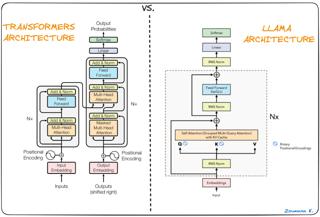
This "consensus recipe" represents years of research and empirical validation, resulting in an architecture that is more stable to train, computationally efficient, and ultimately more performant than its original 2017 counterpart.

Conclusion

In this lesson, we have explored two fundamental improvements to the Transformer block that characterize modern LLMs.

Here are the key takeaways:

• RMSNorm vs. LayerNorm: RMSNorm is a simplified version of LayerNorm that omits the mean-centering step. This makes it computationally faster and more parameter-efficient while delivering comparable performance in modern pre-norm architectures.
• SwiGLU vs. GELU/ReLU: SwiGLU replaces the static nonlinearity of the FFN with a dynamic, input-dependent gating mechanism. This enhances the model's expressive power at a similar parameter budget and consistently leads to better performance.
• Architectural Convergence: These components, along with others like RoPE and pre-norm placement, have become part of a standard, highly-optimized recipe for building powerful decoder-only language models.

You have now completed our module on advanced architectural innovations. You've seen how models scale with Mixture of Experts and how the core Transformer block itself has been refined for maximum efficiency and power.

In our next module, "Decoding Strategies and Inference Optimization," we will shift our focus from training and architecture to inference. Having built and trained these massive models, how do we actually use them to generate coherent, high-quality text? We will explore the algorithms that produce text token-by-token and the optimizations that make this process feasible in real-time applications.