Router Networks and Load Balancing in MoE Layers

The Router: A Learnable Gating Mechanism

At its core, the router is a simple but powerful component: a small, learnable neural network whose job is to calculate an affinity score between an incoming token and each available expert.

The process is straightforward:

1. A token's embedding $x$ (the output from the preceding layer) is fed into the router.
2. The router, which is typically just a single linear layer with a weight matrix $W_{\text{router}}$, computes a vector of logits by multiplying the token embedding by this matrix: $\text{logits}=x\cdot W_{\text{router}}$. This produces one logit per expert.
3. A softmax function is applied to these logits to convert them into a probability distribution, $p=\text{softmax}(\text{logits})$. Each probability $p_i$ represents the router's confidence that expert $i$ is a good choice for processing token $x$.
4. The model then selects the top-k experts with the highest probabilities. Common choices are k=1 (as in Switch Transformers) or k=2 (as in GShard and Mixtral).
5. The final output of the MoE layer is a weighted sum of the outputs from the selected experts, where the weights are their corresponding softmax probabilities.

The following video provides a clear, visual explanation of how the router is implemented and how it uses dot products to generate scores for each expert.

This mechanism is elegant, but it harbors a significant vulnerability. Since the router's weights are learned via backpropagation just like any other parameter, the router will naturally try to optimize for the best performance. This can lead to a problematic dynamic.

The Problem: Routing Collapse

Imagine the start of training. The experts are all initialized randomly, so they are all equally "bad." By chance, the router might send a few more tokens to Expert A and Expert B. As these two experts receive gradient updates, they become slightly better than the others.

This creates a positive feedback loop:

1. Experts A and B perform slightly better.
2. The main task loss (e.g., cross-entropy) decreases when the router sends tokens to A and B.
3. Backpropagation rewards the router for this choice, increasing the probability of routing to A and B in the future.
4. Experts A and B now receive even more tokens, get more updates, and become even better, while the other experts languish.

This phenomenon is known as routing collapse or expert collapse. Left unchecked, the router will learn to send the vast majority of tokens to a very small subset of "favorite" experts. The other experts receive no gradient updates, effectively "dying" and becoming wasted parameters. You end up paying the memory cost for, say, 64 experts but only get the computational benefit of two or three.

To prevent this and ensure that we benefit from the full "mixture" of experts, we need to introduce a mechanism that explicitly encourages the router to spread its load more evenly.

The Solution: Auxiliary Load Balancing Loss

The solution is to add a second loss term to the model's overall training objective. In addition to the primary task loss (${\mathcal{L}}_{\text{task}}$, e.g., cross-entropy for next-token prediction), we add an auxiliary load balancing loss (${\mathcal{L}}_{\text{balance}}$).

The $\alpha$ is a small, tunable hyperparameter that controls the relative importance of the balancing loss. This auxiliary loss acts as a regularizer, penalizing the router for imbalanced token distribution without directly interfering with the model's ability to learn the primary task.

The most common formulation for this loss was introduced in the Switch Transformer paper. It's a clever product of two key quantities calculated over a batch of tokens.

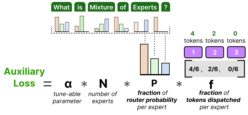
The formula is:

Let's break down the components for a given batch:

• $N$: The total number of experts.
• $f_i$: The fraction of tokens in the batch that were actually assigned to expert $i$. This is a "hard" count based on the top-k selection. For example, if expert $i$ received 100 out of 4000 tokens, $f_i=100/4000=0.025$.
• $P_i$: The average router probability for expert $i$, calculated across all tokens in the batch. This is a "soft" measure of how much the router wanted to send tokens to expert $i$.

The intuition is that the loss penalizes experts that are both frequently chosen ($f_i$ is high) and for which the router is highly confident ($P_i$ is high). The gradient from this loss term pushes down the router logits for overloaded experts, forcing the softmax distribution to spread out more evenly in subsequent steps.

To get a deeper intuition for how this works, we'll walk through a detailed explanation and a concrete numerical example.

Advanced Load Balancing Techniques

The load balancing loss we've just discussed is highly effective, but it's not the only solution, and it introduces a delicate trade-off. If the balancing coefficient $\alpha$ is too high, it can hurt model performance by forcing uniformity at the expense of specialization. If it's too low, routing collapse can still occur. This has motivated an entire field of research into better balancing strategies.

Adding Noise for Stability

One common technique, also from the Switch Transformer paper, is to add random noise to the router's logits during training.

The formula adds a scaled random value to the logits before the top-k selection:

This injection of noise helps prevent the router from becoming overly confident in its choices too early in training and promotes better exploration of all available experts.

Loss-Free Balancing

More recently, models like DeepSeek-V3 have introduced an "auxiliary-loss-free" strategy that elegantly sidesteps the $\alpha$ tuning problem. The core idea is to separate the mechanism for balancing from the calculation of the final output.

1. For Selection: A dynamically updated bias term is added to the router logits. If an expert is overloaded, its bias is decreased. If it's underloaded, its bias is increased. The top-k selection is made based on these biased scores.
2. For Output: The final weighted sum of expert outputs is calculated using the original, unbiased router probabilities.

Because the bias adjustment happens outside of the backpropagation loop, it guides the discrete routing decisions without contaminating the gradients of the main task loss.

The following video segment provides a great overview of this clever approach.

For a comprehensive overview of the historical progression and the variety of balancing strategies developed over the years, from GShard's pioneering work to the latest innovations, the following blog post is an excellent resource. You don't need to read it in full, but skimming the different approaches (like Router Z-loss, GLaM's efficiency focus, etc.) will give you a strong appreciation for the depth of this engineering challenge.

Conclusion

In this lesson, we've dissected the router network, the control center of the MoE layer. We've seen that while its design is simple, its training dynamics can lead to the significant problem of routing collapse.

Here are the key takeaways:

• Router Mechanism: The router is a learnable linear layer that computes a probability distribution over the experts for each token, guiding the selection of the top-k most relevant specialists.
• Routing Collapse: Without intervention, a positive feedback loop during training causes the router to favor a few experts, leading to the underutilization of most of the model's parameters.
• Load Balancing Loss: To counteract this, an auxiliary loss term is added to the training objective. It penalizes the router for imbalanced token distributions, encouraging it to use all experts more evenly.
• Evolving Strategies: The simple load balancing loss is just one of many solutions. The field has evolved to include techniques like adding noise to router logits and sophisticated "loss-free" methods that adjust routing decisions outside the main gradient flow.

You now understand not just what an MoE layer does, but also the critical engineering required to make it learn effectively. In our next and final lesson of this module, we will shift our focus to other modern architectural components that have become standard in state-of-the-art LLMs, comparing them to their original Transformer counterparts.