Understanding LoRA: Efficient Fine-tuning with Low-Rank Adaptations

The Problem with Scale: Why Full Fine-Tuning is Impractical

Before diving into LoRA's mechanics, it's crucial to solidify our understanding of the problem it solves. Full fine-tuning, as discussed, updates the entire weight matrix $\Phi$ to ${\Phi }_0+\Delta \Phi$. For a model like GPT-3 175B, this means:

• Massive Storage: Each fine-tuned task requires storing a new set of weights, which can be hundreds of gigabytes or even terabytes. Deploying dozens of custom models becomes a logistical nightmare.
• High Computational Cost: Backpropagation through billions of parameters and updating their corresponding optimizer states (like in Adam) requires a substantial amount of GPU memory and processing time.
• Slow Task-Switching: In a production environment where you might need to serve multiple fine-tuned models, swapping terabytes of weights in and out of GPU VRAM is unacceptably slow.

These challenges created a strong need for a method that could adapt a model without creating a full copy.

The Core Hypothesis: Weight Updates Have a Low Intrinsic Rank

The key insight behind LoRA comes from an observation about the nature of neural networks. While a pre-trained model's weight matrices are typically full-rank, researchers hypothesized that the change in those weights during adaptation, $\Delta W$, does not need to be. Instead, they proposed that this update matrix has a low "intrinsic rank".

From your linear algebra studies, you'll recall that the rank of a matrix is the number of linearly independent columns (or rows) it contains. A low-rank matrix is one where many columns are redundant linear combinations of a few basis columns. The LoRA hypothesis is that the essential information required to adapt a model to a new task can be captured in a very low-dimensional update, even if the weight matrices themselves are high-dimensional.

Instead of learning a massive, potentially redundant matrix $\Delta W$ with $d\times k$ parameters, what if we could learn a much smaller representation that effectively accomplishes the same goal?

The LoRA Mechanism: Low-Rank Decomposition

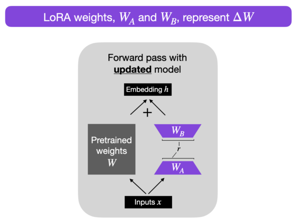
This is where matrix decomposition comes into play. LoRA constrains the update matrix $\Delta W$ by representing it as the product of two much smaller matrices: $B$ and $A$.

For a pre-trained weight matrix $W_0\in {\mathbb{R}}^{d\times k}$, the update is not learned directly. Instead, we have:

where $B\in {\mathbb{R}}^{d\times r}$ and $A\in {\mathbb{R}}^{r\times k}$. The hyperparameter $r$ is the rank of the decomposition, and it is typically very small (e.g., 8, 16, 32), satisfying $r\ll \min (d,k)$.

During training:

1. The original weights $W_0$ are frozen and do not receive gradient updates.
2. The new, smaller matrices $A$ and $B$ are the only trainable parameters.

The forward pass through a LoRA-modified layer is then modified. For an input $x$, the output $h$ becomes:

This can be seen as a parallel path that adds a small, learned "correction" to the output of the original frozen layer.

Analyzing the Parameter Efficiency

Let's quantify the savings.

• Full Fine-Tuning: Learning $\Delta W$ requires training $d\times k$ parameters.
• LoRA: Learning $A$ and $B$ requires training $(d\times r)+(r\times k)=r(d+k)$ parameters.

Consider a typical layer in an LLM where $d=4096$ and $k=4096$.

• A full update requires $4096\times 4096\approx 16.7$ million parameters.
• With a LoRA rank of $r=8$, we only need to train $8\times (4096+4096)=65,536$ parameters.

This represents a parameter reduction of over 99.5% for this single layer, demonstrating the immense efficiency of the approach.

As you read, note the clever initialization strategy: matrix $B$ is initialized to all zeros, while $A$ is initialized with a random Gaussian distribution. This ensures that at the beginning of training, $\Delta W=BA=0$. The model starts exactly as the pre-trained model, and adaptation begins gradually as $A$ and $B$ are updated.

The Complete Picture: Training and Inference

The full LoRA process is elegant in its simplicity.

1. During Training: We keep the base model frozen and only train the small A and B matrices for each selected layer (typically the attention layers). This drastically reduces the memory needed for gradients and optimizer states, allowing fine-tuning on consumer-grade hardware.

2. For Inference: Because the LoRA update is purely additive, we can merge the trained weights back into the main model. We compute $W_{\text{merged}}=W_0+BA$ once and save this new matrix. The model can then be deployed as a standard network with a single weight matrix per layer. This means LoRA introduces zero additional inference latency compared to a non-fine-tuned model, a major advantage over other PEFT methods like adapters, which add extra layers to the architecture.

The Mathematical Formulation Summarized

To consolidate the core mathematics, let's review the formulation.

The article also introduces a scaling factor, $\alpha$, which is often applied to the update: $h=W_{0}x+\frac{\alpha }{r}BAx$. This scaling helps to normalize the magnitude of the adaptation when you experiment with different values of rank $r$, making hyperparameter tuning more stable.

Conclusion

In this lesson, we've moved from the brute-force approach of full fine-tuning to the surgical precision of Low-Rank Adaptation. We have seen how a simple hypothesis about the nature of model adaptation, combined with a standard linear algebra technique, leads to a remarkably efficient and effective fine-tuning method.

Here are the key takeaways:

• Motivation: LoRA was developed to overcome the prohibitive storage and computational costs of fully fine-tuning massive language models for multiple tasks.
• Core Idea: It is based on the hypothesis that the change in model weights during fine-tuning has a low "intrinsic rank."
• Mechanism: Instead of updating the full weight matrix $W_0$, LoRA freezes $W_0$ and injects a trainable, low-rank update represented by the product of two small matrices, $\Delta W=BA$.
• Parameter Efficiency: This decomposition drastically reduces the number of trainable parameters (e.g., from millions to thousands), making fine-tuning much more accessible.
• No Inference Latency: After training, the low-rank matrices can be merged with the original weights ($W_{\text{merged}}=W_0+BA$), meaning there is no performance overhead during inference.

You now understand not just that LoRA is efficient, but why it is efficient, grounded in the concept of low-rank matrix decomposition.

In our next lesson, we will formalize the comparison between full fine-tuning and PEFT. We'll analyze the trade-offs between methods like LoRA and full fine-tuning across dimensions like computational cost, memory usage, storage, and final model performance, giving you a complete framework for deciding which adaptation strategy to use in different scenarios.