Layer Normalization's Role in Transformer Stability

The Problem of Shifting Scales: Internal Covariate Shift

Deep neural networks learn by passing activations forward and gradients backward. Each layer is constantly updating its weights, which in turn changes the distribution of the outputs it produces. For the next layer in the stack, this means its input distribution is constantly changing during training. This phenomenon is called internal covariate shift.

Imagine a series of complex systems in a pipeline, where each system is trying to calibrate itself based on the output of the previous one. If the output characteristics of each system are constantly and erratically changing, the downstream systems will struggle to find a stable operating point. In a neural network, this forces each layer to continually adapt to a moving target, slowing down and destabilizing the learning process.

Normalization aims to solve this by standardizing the inputs to each layer, ensuring they have a consistent mean and variance. This provides a more stable foundation for the layer to learn from, much like how standardizing an API contract allows different services to interact reliably.

To get a clear intuition for this, please watch the following video segment. It provides an excellent analogy and visual explanation for why normalization is needed in deep networks.

Normalizing Activations: Layer Norm vs. Batch Norm

So, how do we normalize the activations inside a network? A very common technique is Batch Normalization (BN). For each neuron (or feature), BN computes the mean and standard deviation across all examples in the current batch. It then normalizes the neuron's activation for each example using these batch-wide statistics.

However, this approach presents a significant problem for sequence data in Transformers. Sentences in a batch have different lengths. To process them together, we pad the shorter sentences with special "padding" tokens. If we were to use Batch Normalization, the statistics for each feature would be contaminated by these artificial padding values, skewing the mean and variance. The amount of skew would also change from batch to batch depending on the lengths of the sentences, making the normalization itself unstable.

The solution is Layer Normalization (LN). Instead of normalizing across the batch, LN normalizes across the features within a single training example. For a given token's embedding vector, Layer Normalization calculates the mean and standard deviation of all the values in that vector alone. This makes it completely independent of other examples in the batch and immune to the problems of padding.

The following video segment walks through this exact distinction, explaining why Batch Normalization is ill-suited for Transformers and how Layer Normalization resolves the issue.

The Mechanics of Layer Normalization

The mathematical formulation for Layer Normalization is direct. For an input vector $x$ (representing a single token's embedding of dimension $d$), the normalized vector $\hat{x}$ is calculated. Then, two learnable parameter vectors, a scale $\gamma$ (gamma) and a bias $\beta$ (beta), are applied.

The full operation is:

Where:

• $\mu$ is the mean of the elements in vector $x$: $\mu =\frac{1}{d}{\sum }_{i=1}^d{x}_i$
• ${\sigma }^2$ is the variance of the elements in vector $x$: ${\sigma }^2=\frac{1}{d}{\sum }_{i=1}^d(x_i-\mu {)}^2$
• $ϵ$ is a small constant (e.g., $10^{-5}$) added for numerical stability to prevent division by zero.
• $\gamma$ and $\beta$ are learnable parameter vectors of the same dimension as $x$. They are initialized to 1 and 0, respectively.
• $\odot$ denotes element-wise multiplication.

The purpose of $\gamma$ and $\beta$ is crucial. While normalization provides stability, it also constrains the representational power of the layer. By introducing these learnable parameters, the network can scale and shift the normalized output. In the extreme case, it can learn to set $\gamma$ to $\sqrt{{\sigma }^2+ϵ}$ and $\beta$ to $\mu$, effectively undoing the normalization and recovering the original activations. This gives the model the flexibility to decide, through training, the optimal degree of normalization for each layer.

To see this formula in action, the next video provides a concrete numerical walkthrough.

Pre-LN vs. Post-LN: A Key to Stability

We now understand what Layer Normalization does. However, where it is placed has a profound impact on training stability. This is a perfect example of how a subtle architectural choice can have major systemic effects.

There are two primary configurations:

1. Post-Layer Normalization (Post-LN): LayerNorm(x + Sublayer(x))
   This was the original design from the "Attention is All You Need" paper. The input x passes through the sub-layer (e.g., attention), the residual connection is added, and then the result is normalized.

2. Pre-Layer Normalization (Pre-LN): x + Sublayer(LayerNorm(x))
   In this design, the input x is first normalized and then passed to the sub-layer. The residual connection is added afterward.

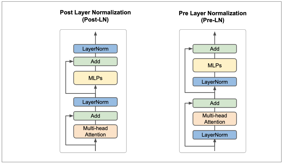
While Post-LN was used in early Transformers, it was discovered to be difficult to train. The optimization process is sensitive and often requires a carefully tuned learning rate warm-up: starting with a very small learning rate and gradually increasing it. Without this, training can diverge.

The reason, as explored in the paper "On Layer Normalization in the Transformer Architecture" by Xiong et al., is that in Post-LN models, the gradients flowing back to the parameters can be very large, especially in the upper layers. A large learning rate applied to these explosive gradients causes instability. The warm-up stage acts as a workaround, taming the updates until the model settles.

Conversely, the Pre-LN architecture provides a much more stable training dynamic. By normalizing the input before it enters the sub-layer, the activations are kept under control throughout the forward pass. This, in turn, leads to well-behaved, stable gradients during the backward pass, right from the start of training. As a result, Pre-LN Transformers are less sensitive to initialization and often do not require a learning rate warm-up, allowing for faster and more robust training. This is why Pre-LN has become the de facto standard in most modern LLMs.

The following reading from the Xiong et al. paper will guide you through the theoretical and empirical evidence for this critical finding. Your background in calculus will be valuable for appreciating the argument about gradient norms.

Conclusion

In this lesson, we have dissected the "Norm" component that works in tandem with the residual connections we studied previously. You now understand that Layer Normalization is not merely an add-on but a critical mechanism for ensuring the stability and efficiency of training deep Transformers.

Here are the key takeaways:

• Purpose: Layer Normalization stabilizes training by combatting internal covariate shift, ensuring that the input to each layer maintains a consistent distribution (zero mean, unit variance).
• Mechanism: It operates on a per-example basis, normalizing across the feature dimension. This makes it ideal for variable-length sequence data, unlike Batch Normalization.
• Flexibility: The learnable $\gamma$ (scale) and $\beta$ (shift) parameters allow the model to dynamically control the extent of normalization, preserving representational power.
• Stability and Architecture: The placement of LayerNorm is crucial. Pre-LN architectures (x + Sublayer(LayerNorm(x))) produce more stable gradients from initialization, are easier to train, and often remove the need for learning rate warm-up. This is a significant improvement over the original Post-LN design and is standard in modern LLMs.

We have now assembled all the pieces of the two main sub-layers within a Transformer block: Multi-Head Attention and the Position-wise Feed-Forward Network, each wrapped in a residual connection and a layer normalization step. In the next lessons, we will trace the complete data flow through these components to see how they work together to process information.