Multi-Head Attention: Data Flow with Residuals and Normalization

Introduction

In our previous lessons, we've carefully assembled the foundational components of a Transformer block. We've explored Multi-Head Attention (MHA) as the core mechanism for processing relationships within a sequence. We've also seen how residual connections provide a direct "highway" for gradients and how Layer Normalization stabilizes the entire learning process. Now, it's time to connect these pieces and see how they function as a cohesive unit.

This lesson focuses on tracing the precise path that data takes as it flows through the first major component of a Transformer block: the Multi-Head Attention sub-layer. We will see how an input tensor is processed by the attention mechanism and then integrated back with its original form via the "Add & Norm" step. Building on our last discussion, we will prioritize the modern, more stable Pre-Layer Normalization (Pre-LN) architecture, while also examining the original Post-LN design to ensure you can confidently interpret various implementations you'll encounter in papers and codebases.

The Modern Standard: The Pre-LN Attention Sub-layer

Most modern Large Language Models have adopted the Pre-LN architecture due to the superior training stability we discussed previously. The data flow is logical: first, we stabilize the input, then we process it with attention, and finally, we reintegrate the processed information.

Let's trace the journey of an input tensor $X$ with dimensions [batch_size, seq_len, d_model].

The overall flow for a Pre-LN sub-layer is: Output = Input + Sublayer(LayerNorm(Input)).

Here is the step-by-step breakdown:

Pre-Normalization: The input tensor $X$ is first passed through a Layer Normalization module. This step standardizes the feature distribution for each token before it's used in the attention calculation, which is key to maintaining stable activations.
$X_{norm} = LayerNorm (X)$
The resulting tensor, $X_{norm}$ , has the exact same dimensions as $X$ .
Multi-Head Attention: The normalized tensor, $X_{norm}$ , is then used as the source for the Query, Key, and Value matrices. In this self-attention sub-layer, all three are derived from the same input.
$Z = MultiHeadAttention (Q = X_{norm}, K = X_{norm}, V = X_{norm})$
The output of the MHA module, $Z$ , also retains the dimensions [batch_size, seq_len, d_model]. It represents the re-weighted and aggregated information from the sequence.
Residual Connection: The output of the MHA module, $Z$ , is added back to the original, un-normalized input tensor $X$ . A dropout layer is typically applied to $Z$ for regularization before the addition.
$X_{output} = X + Dropout (Z)$
This final tensor, $X_{output}$ , is the result of the entire sub-layer. It carries the original positional information and identity from $X$ , now enriched with the contextual understanding captured by $Z$ . This tensor is then passed to the next sub-layer in the Transformer block.

A Deeper Look into the Multi-Head Attention Step

Step 2 is where the core computation happens. The following video provides a detailed mathematical and visual walkthrough of how the Multi-Head Attention module takes an input tensor and produces the output $Z$ . As you watch, focus on the flow of matrices and the transformation of their dimensions.

Attention is all you need (Transformer) - Model explanation (including math), Inference and Training

This video from Umar Jamil provides a clear, step-by-step explanation of the Multi-Head Attention mechanism, detailing how the Q, K, and V matrices are created, split, processed in parallel, and reassembled.

Please watch the segment from Multi-head attention. Pay close attention to how the input tensor with dimension (sequence, d_model) is transformed into Query, Key, and Value matrices, then split into multiple heads along the d_model dimension. Note how the output of each head is concatenated and projected back to the original d_model dimension.

The Original Architecture: Post-LN Sub-layer

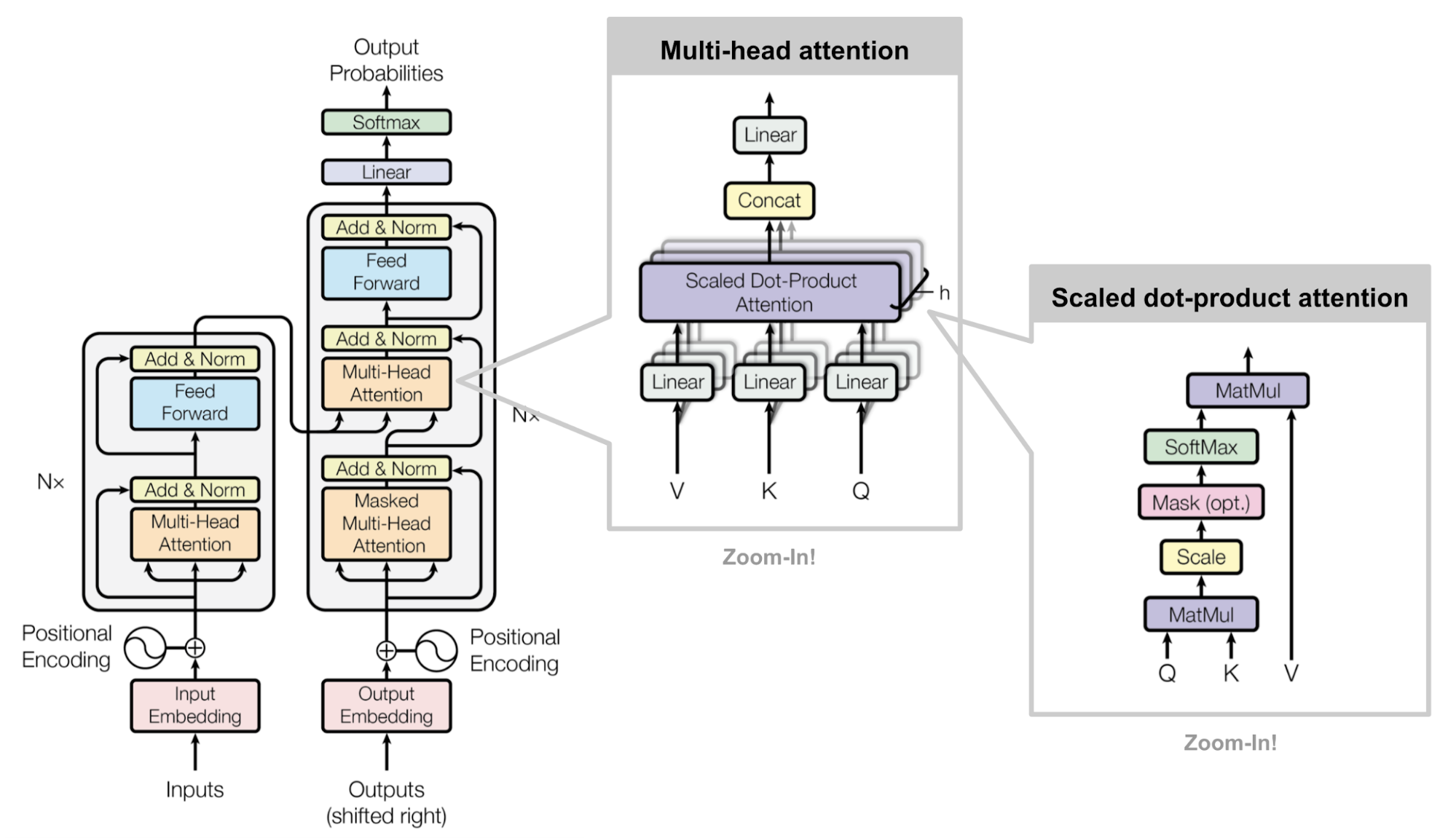
While Pre-LN is the current standard, the original "Attention is All You Need" paper and many subsequent tutorials use a Post-LN architecture. It's crucial to recognize this pattern.

The flow for a Post-LN sub-layer is: Output = LayerNorm(Input + Sublayer(Input)).

Multi-Head Attention: The MHA module operates directly on the raw input tensor $X$ . $Z = MultiHeadAttention (Q = X, K = X, V = X)$
Residual Connection and Normalization: The output $Z$ is added to the input $X$ , and the result of this addition is then passed through Layer Normalization. $X_{output} = LayerNorm (X + Dropout (Z))$

Notice the critical difference: in Post-LN, the normalization happens after the residual connection, acting on a potentially high-variance sum. In Pre-LN, it happens before the main sub-layer, ensuring the attention mechanism always receives a clean, stable input.

The following resources provide excellent examples of the Post-LN architecture in both explanation and code. As you study them, identify the specific lines that reveal the Post-LN data flow.

Tutorial 6: Transformers and Multi-Head Attention

This tutorial from the UvA Deep Learning course provides a clear implementation of a Transformer Encoder block following the original Post-LN design.

First, read the section on the encoder architecture. Note the formula given: LayerNorm(x + Multihead(x,x,x)). Next, examine the provided code for the EncoderBlock. In the forward method, locate these two lines: Attention part Add & Norm This sequence—attention, then add, then normalize—is the hallmark of a Post-LN block.

Here is a diagram from the popular "Illustrated Transformer" blog post, which also depicts the Post-LN flow. The "Add & Norm" box is a single conceptual unit where the output of the MHA block is added to the skip connection, and the sum is then normalized.

This diagram shows the classic encoder-decoder structure. Within each encoder and decoder block, you can see the Multi-Head Attention followed by an "Add & Norm" layer, which is characteristic of the Post-LN design.

Synthesis: Comparing the Data Flows

The data tensor maintains its shape [batch_size, seq_len, d_model] throughout its journey in this sub-layer, regardless of the architecture. However, the order of operations is fundamentally different, with significant implications for training dynamics.

Here's a side-by-side comparison:

Step	Pre-LN Flow (`x + Sublayer(Norm(x))`)	Post-LN Flow (`Norm(x + Sublayer(x))`)
1	$X_{norm} = LayerNorm (X)$	$Z = MHA (X, X, X)$
2	$Z = MHA (X_{norm}, X_{norm}, ...)$	$X_{sum} = X + Dropout (Z)$
3	$X_{output} = X + Dropout (Z)$	$X_{output} = LayerNorm (X_{sum})$

Your DevOps background gives you an appreciation for stable, predictable pipelines. The Pre-LN architecture can be seen as an improvement that stabilizes the data processing pipeline within the Transformer, making the entire system more robust and easier to train—a direct parallel to refining a CI/CD workflow for greater reliability.

Conclusion

In this lesson, we have traced the complete data flow through the Multi-Head Attention sub-layer, the first of two major components in a Transformer block.

Key takeaways include:

The sub-layer's function is to take an input sequence representation $X$ and produce an output $X_{output}$ of the same shape, enriched with contextual information.
This is achieved by combining three operations: Multi-Head Attention, a residual connection, and Layer Normalization.
The Pre-LN architecture (x + MHA(LayerNorm(x))) is the modern standard due to its superior training stability. It normalizes the data before the attention computation.
The Post-LN architecture (LayerNorm(x + MHA(x))) was used in the original Transformer and is common in many tutorials. It normalizes after the residual connection.
Understanding both patterns is essential for correctly interpreting different Transformer implementations in research and practice.

We have now successfully navigated the first half of a Transformer block. In our next lesson, we will trace the data flow through the second half: the Position-wise Feed-Forward Network. By the end, you will have a complete picture of how a single Transformer block processes information from input to output.