Direct Preference Optimization (DPO): A Reward-Model-Free RLHF Alternative

In our last lesson, we navigated the complex machinery of Proximal Policy Optimization (PPO), the reinforcement learning engine that powers the final stage of the RLHF alignment process. You saw how PPO, through an intricate system of four models and carefully engineered safeguards, manages to optimize a language model against a learned reward signal. While powerful, its complexity is undeniable, which naturally leads to the question: is there a simpler way?

Today, we will explore a groundbreaking and elegant answer to that question: Direct Preference Optimization (DPO). This lesson will show how DPO reframes the alignment problem, allowing us to achieve the same goal as RLHF but without an explicit reward model and without the entire reinforcement learning loop. By the end of this lesson, you will understand the mathematical derivation that makes DPO possible and appreciate why it has become such a popular and powerful alternative for LLM alignment.

The Problem, Revisited

Let's begin by recalling the fundamental objective of the RLHF alignment process. We want to find an optimal policy, $π$ , that maximizes the expected reward from our reward model, $r (x, y)$ , while not straying too far from our initial Supervised Fine-Tuned (SFT) model, which we call the reference policy, $π_{ref}$ . This is a constrained optimization problem, formulated as:

π max E_{x \sim D, y \sim π (y ∣ x)} [r (x, y) - β D_{K L} (π (y ∣ x) ∣∣ π_{ref} (y ∣ x))]

Here, $D_{K L}$ is the Kullback-Leibler divergence that penalizes the policy for deviating from the reference, and $β$ is a hyperparameter controlling the strength of this penalty.

The previous lesson showed that PPO is an iterative, algorithmic approach to solving this. DPO starts from a different, more analytical premise: what if this optimization problem has a closed-form solution?

The Four Steps of DPO

The core insight of DPO is a brilliant piece of mathematical substitution that transforms the complex RL problem into a simple classification problem. The entire derivation can be understood in four conceptual steps, as illustrated below. We will walk through each one.

This flowchart outlines the key logical steps in deriving the DPO loss. It begins with the RLHF objective, finds its optimal solution, re-expresses it as an implicit reward, plugs this into the Bradley-Terry preference model, and finally arrives at a trainable loss function by training an LLM to match the resulting preference distribution.

Step 1: Find the Optimal Solution for the RLHF Objective

It turns out that the constrained optimization problem above has an exact analytical solution. The policy $π^{*}$ that maximizes this objective can be written as:

π^{*} (y ∣ x) = \frac{1}{Z ( x )} π_{ref} (y ∣ x) exp (\frac{1}{β} r (x, y))

where $Z (x)$ is a normalization constant called the partition function, defined as:

Z (x) = y \sum π_{ref} (y ∣ x) exp (\frac{1}{β} r (x, y))

This equation tells us that the optimal policy is simply the reference policy, re-weighted by the exponentiated reward. Responses that get a higher reward are made exponentially more likely.

However, we can't use this solution directly. The partition function $Z (x)$ requires summing over the rewards of all possible completions $y$ , which is computationally intractable for any non-trivial language model.

Step 2: Rearrange to Yield an Implicit Reward Function

Here comes the first key maneuver of DPO. Instead of trying to compute $π^{*}$ from $r$ , what if we rearrange the equation to express the reward function $r$ in terms of $π^{*}$ ? A bit of algebraic manipulation (applying a logarithm and isolating $r (x, y)$ ) gives us:

r (x, y) = β lo g (\frac{π ^{*} ( y ∣ x )}{π _{ref} ( y ∣ x )}) + β lo g (Z (x))

This is a profound statement. It defines the reward function in terms of the log-probability ratio between the optimal and reference policies. It implies that the reward is implicitly encoded in the policy itself. This insight is the origin of the DPO paper's subtitle: "Your Language Model is Secretly a Reward Model". We still have the intractable $lo g (Z (x))$ term, but we are one step closer.

Step 3: Plug the Implicit Reward into the Bradley-Terry Model

Recall from our lesson on reward modeling that we use the Bradley-Terry model to link rewards to human preferences. It defines the probability that a human would prefer a "winning" completion $y_{w}$ over a "losing" completion $y_{l}$ as a function of their rewards:

P (y_{w} ≻ y_{l} ∣ x) = σ (r (x, y_{w}) - r (x, y_{l}))

where $σ$ is the sigmoid function.

Now, we substitute our new expression for the implicit reward function from Step 2 into the Bradley-Terry model. This is the crucial step where the magic happens.

When we compute the difference $r (x, y_{w}) - r (x, y_{l})$ , the term $β lo g (Z (x))$ appears in both expressions. Since this term depends only on the prompt $x$ and not the completion $y$ , it is identical for both $y_{w}$ and $y_{l}$ , and therefore cancels out perfectly!

The video "Direct Preference Optimization (DPO) explained" by Umar Jamil provides an excellent, detailed walkthrough of this derivation.

Direct Preference Optimization (DPO) explained: Bradley-Terry model, log probabilities, math

This video methodically derives the DPO loss, starting from the same RLHF objective we've been discussing. It clearly explains each step, including the intractable partition function and its eventual cancellation.

First, watch the section on the analytical solution. This covers Steps 1 and 2 of our derivation, explaining the optimal policy \pi^* and how it's rearranged to define the implicit reward function, highlighting the problem with the Z(x) term. Next, watch the key substitution step. This corresponds to our Step 3, showing exactly how plugging the implicit reward into the Bradley-Terry model causes the intractable Z(x) terms to cancel out.

Step 4: Train an LLM to Match the Preference Distribution

After the cancellation, we are left with a clean, computable expression for the preference probability under the optimal policy:

P (y_{w} ≻ y_{l} ∣ x) = σ (β lo g \frac{π ^{*} ( y _{w} ∣ x )}{π _{ref} ( y _{w} ∣ x )} - β lo g \frac{π ^{*} ( y _{l} ∣ x )}{π _{ref} ( y _{l} ∣ x )})

We don't know the optimal policy $π^{*}$ , but we want to train our policy $π_{θ}$ to become it. So, we replace $π^{*}$ with $π_{θ}$ and treat this equation as our goal. We want to maximize the probability of the observed human preferences in our dataset $D$ . This is a standard maximum likelihood estimation task, for which the loss function is the negative log-likelihood of the data.

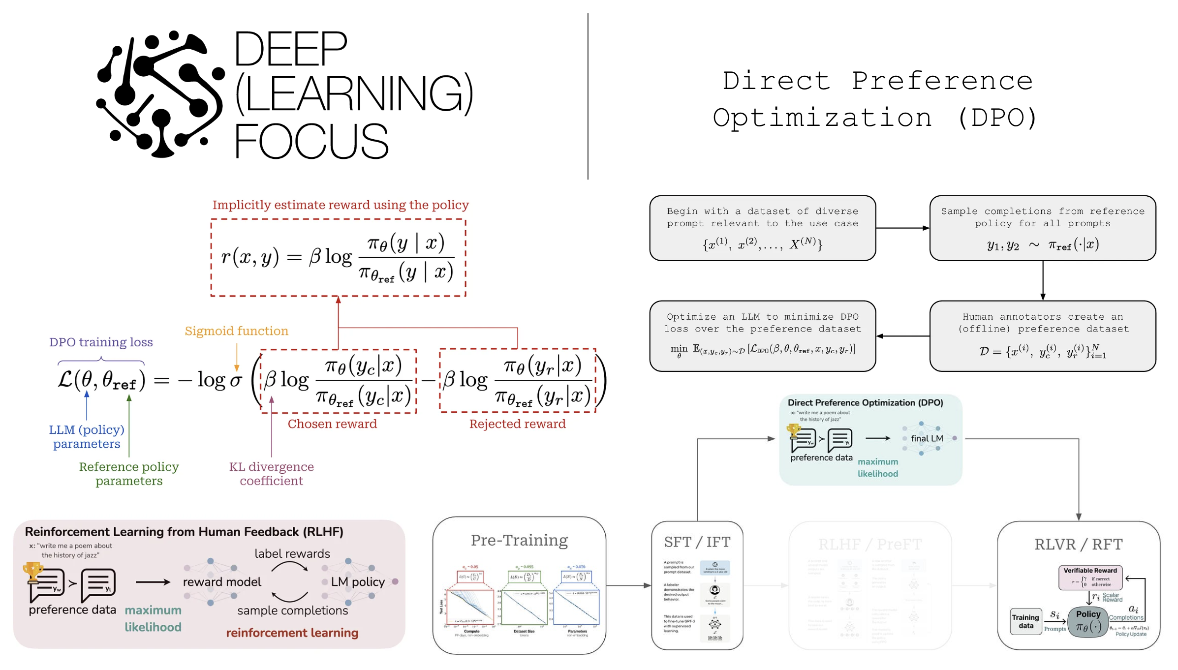
This gives us the final DPO loss function:

L_{DPO} (π_{θ}; π_{ref}) = - E_{(x, y_{w}, y_{l}) \sim D} [lo g σ (β lo g \frac{π _{θ} ( y _{w} ∣ x )}{π _{ref} ( y _{w} ∣ x )} - β lo g \frac{π _{θ} ( y _{l} ∣ x )}{π _{ref} ( y _{l} ∣ x )})]

This might look complex, but it's fundamentally a binary cross-entropy loss. We have transformed the multi-stage, four-model RLHF problem into a single-stage classification problem on pairs of completions, trainable with standard gradient descent.

This infographic provides a concise summary of Direct Preference Optimization (DPO). It highlights the core DPO training loss, illustrates how the implicit reward is estimated using the policy and reference models, and contrasts the simpler DPO workflow (bottom) with the more complex multi-stage RLHF process (middle-left).

Building Intuition for the DPO Loss

Let's dissect the loss function to understand what it's actually doing during training. The core term inside the sigmoid is the difference between two implicit rewards:

r^_{θ} (x, y) = β lo g \frac{π _{θ} ( y ∣ x )}{π _{ref} ( y ∣ x )}

This implicit reward, $r^_{θ}$ , measures how much more likely the current policy $π_{θ}$ is to generate response $y$ compared to the reference policy $π_{ref}$ . The DPO loss aims to maximize the difference $r^_{θ} (x, y_{w}) - r^_{θ} (x, y_{l})$ .

To achieve this, the optimization must:

Increase $lo g π_{θ} (y_{w} ∣ x)$ : Make the chosen completions more likely.
Decrease $lo g π_{θ} (y_{l} ∣ x)$ : Make the rejected completions less likely.

This aligns our model directly with the preference data. For a more formal analysis, we can examine the gradient of the DPO loss with respect to the model parameters $θ$ .

Deriving the DPO Loss from First Principles - Hugging Face

The Hugging Face blog post "Deriving the DPO Loss from First Principles" provides a clear derivation of the gradient of the DPO objective. This will give us a precise understanding of the update rule.

Please read the subsection Analyzing the Gradient Update. Focus on the final boxed equation for the gradient and the interpretation of its components.

As the reading shows, the gradient update can be expressed as:

\nabla_{θ} L_{DPO} \propto - β [σ (r^_{θ} (x, y_{l}) - r^_{θ} (x, y_{w}))] (\nabla_{θ} lo g π_{θ} (y_{w} ∣ x) - \nabla_{θ} lo g π_{θ} (y_{l} ∣ x))

This reveals a crucial third component:
3. Dynamic Weighting: The term $σ (r^_{θ} (x, y_{l}) - r^_{θ} (x, y_{w}))$ acts as a dynamic weight on the update. If the model already assigns a much higher implicit reward to $y_{w}$ (i.e., the reward difference is large and negative), this sigmoid term becomes close to zero, and the update is small. Conversely, if the model incorrectly prefers the rejected completion $y_{l}$ , this weight becomes large, focusing the training on the "hard" examples it is currently getting wrong. This makes the learning process highly efficient.

DPO vs. PPO: A Simpler Path to Alignment

The elegance of DPO lies in what it removes. Compared to the PPO-based RLHF pipeline:

No Explicit Reward Model: We no longer need to train and store a separate reward model. The reward is implicitly defined by the policy being trained.
No Reinforcement Learning: The complex, often unstable RL training loop is gone. DPO is a simple supervised learning problem.
No Sampling During Training: PPO requires generating samples from the policy "in the loop" to explore the environment. DPO works offline on a static preference dataset.
Fewer Models: DPO training requires only two models in memory: the policy being trained ( $π_{θ}$ ) and the frozen reference policy ( $π_{ref}$ ). PPO requires four: the actor, the critic, the reward model, and the reference policy. This significantly reduces the hardware requirements.

By cleverly reparameterizing the RLHF objective, DPO provides a more stable, computationally cheaper, and simpler path to achieving the same alignment goal.

Conclusion

In this lesson, we have unraveled the theory behind Direct Preference Optimization. You've seen how a sequence of mathematical steps can transform a complex reinforcement learning problem into a straightforward supervised learning task, bypassing the need for an explicit reward model and the instabilities of RL.

Here are the key takeaways:

The standard RLHF objective has an exact analytical solution for the optimal policy, but it is computationally intractable due to a partition function $Z (x)$ .
DPO's central insight is to re-express the reward function in terms of the policy and then substitute this into the Bradley-Terry preference model.
This substitution causes the intractable partition function to cancel out, leaving a clean, computable objective.
The final DPO loss is equivalent to a binary cross-entropy loss on preference pairs, which aims to increase the log-probability of preferred responses and decrease the log-probability of rejected responses.
The gradient analysis reveals that DPO dynamically weights updates to focus on examples where the model's current preferences are incorrect.
This approach eliminates the need for an explicit reward model and the complexities of RL, making DPO a more stable, efficient, and accessible alignment technique than PPO-based RLHF.

The development of DPO represents a significant step forward in making powerful alignment techniques more accessible to the broader research community. In our final module, we will shift our focus from training and adaptation to the practical challenges of evaluating and deploying these massive models in the real world.

Recommended resources