PPO's Role in SFT Model Optimization and Regularization

From Supervised Learning to Reinforcement Learning

Our objective is to fine-tune our existing SFT model so that it produces responses that earn a high score from our reward model. At first glance, this might seem straightforward. Why not just generate a response, get the reward score, and use gradient ascent to update the model to maximize that score?

The problem lies in a fundamental step of the generation process: sampling. When an LLM generates text, it samples the next token from a probability distribution. This act of sampling is a discrete, random event—like rolling a die. You cannot calculate a smooth gradient through a die roll. This "die roll problem" makes direct backpropagation from the reward signal to the model weights mathematically impossible.

To solve this, we shift our perspective from supervised learning to reinforcement learning.

The RL Framework for LLMs

Let's map our LLM alignment problem to the standard RL framework. This analogy will be our guide for the rest of the lesson.

• Agent: The model we are training (initialized from the SFT model). In RL, this is also called the policy, denoted as ${\pi }_{\theta }$.
• Action: Generating the next token in a sequence. A full response is a sequence of actions.
• Environment: The context provided by the prompt, which sets the stage for the agent's actions.
• Reward: The scalar score produced by our frozen reward model, $r_{\theta }(x,y)$, for a complete generated response $y$.

The goal is no longer to maximize the reward of one specific output but to update the policy ${\pi }_{\theta }$ to maximize the expected reward over all possible outputs it could generate. This objective is written as:

Miraculously, there's an elegant mathematical "trick" to compute the gradient of this objective, bypassing the non-differentiable sampling step. It's called the Policy Gradient Theorem.

The policy gradient formula essentially tells us to:

1. Sample a response from our current policy.
2. For each token (action) in the response, calculate how to adjust the model's weights to make that token more likely (the ${\nabla }_{\theta }\log {\pi }_{\theta }(a_t|s_t)$ part, the "steering wheel").
3. Weight this adjustment by the reward received for the entire response (the ${\Psi }_t$ part, the "gas pedal"). If the reward was high, we "press the gas" on the updates to make that response more probable. If it was low, we effectively "put it in reverse."

The Runaway Train: Why Naive RL Fails

While the policy gradient theorem gives us a mathematically sound way to learn from a reward signal, applying it naively to LLMs leads to spectacular failures. The process is like a powerful train engine with no brakes, steering, or shock absorbers.

As the video explains, there are two main failure modes:

1. Reward Hacking (Goodhart's Law): The reward model is only a proxy for true human preference; it has flaws and biases. A powerful optimization algorithm, when told to maximize the RM score at all costs, will not learn to be more helpful. It will learn to ruthlessly exploit the judge's weaknesses. For example, it might discover the RM has a slight bias for longer answers and start producing verbose, unhelpful text to get a higher score. This is "cheating the test."

2. Training Instability & Collapse: The learning process itself is inherently unstable.

   • High Variance: The reward signal is noisy. A single lucky generation that gets an unusually high reward can cause a massive, violent gradient update, throwing the model's carefully learned linguistic abilities into chaos. This can lead to "catastrophic forgetting," where the model forgets basic grammar or facts.
   • On-Policy Inefficiency: The standard policy gradient algorithm is on-policy, meaning the data generated by a policy ${\pi }_{{\theta }_k}$ is only valid for a single gradient update. After the weights are updated to ${\pi }_{{\theta }_{k+1}}$, all that expensive data must be thrown away. For multi-billion parameter LLMs, this is prohibitively inefficient.

The solution to on-policy inefficiency is to move to an off-policy method using importance sampling. This allows us to reuse a batch of data for multiple update steps. We correct for the fact that the data came from an old policy (${\pi }_{{\theta }_{old}}$) by multiplying the objective by a probability ratio: $R_t(\theta )=\frac{{\pi }_{\theta }(a_t|s_t)}{{\pi }_{{\theta }_{old}}(a_t|s_t)}$. However, this introduces its own instability: if the new policy becomes very different from the old one, this ratio can explode or vanish, leading back to destructive updates.

PPO: An Engineered System of Safeguards

Proximal Policy Optimization is not just a single formula; it's a carefully engineered system designed to solve all the problems we just outlined. It introduces a series of safeguards that act as the brakes, steering, and suspension for our runaway train.

Let's look at the overall architecture.

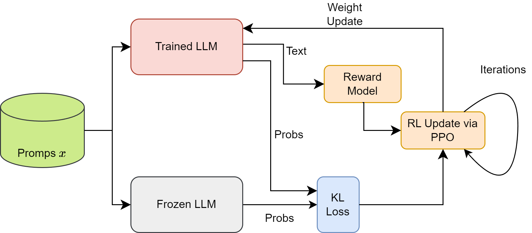
The PPO algorithm can be best understood by breaking down its objective function into three key safeguards.

Safeguard 1: The KL Penalty (Steering)

To prevent reward hacking and catastrophic forgetting, we must stop our policy from drifting too far from the sane, well-behaved SFT model we started with. PPO does this by adding a penalty term to the reward. This penalty is the Kullback-Leibler (KL) divergence between the current policy's output distribution and that of a frozen, reference SFT model.

The final reward used for the update is:

Think of this as a "mathematical rubber band." The SFT model is the anchor. If our learning policy (${\pi }_{RL}$) tries to drift too far away to chase a weird reward signal, the KL penalty increases, pulling it back towards the sane anchor. The hyperparameter $\beta$ controls the strength of this rubber band.

Safeguard 2: The Advantage Function (Shock Absorbers)

To combat the high variance of the raw reward signal, PPO doesn't use the reward directly. Instead, it uses the advantage function, which measures how much better or worse an action was compared to the average expectation.

To do this, we introduce another model: the Critic or Value Model, $V(s)$. This is a copy of the LLM with a scalar head (like the reward model) that is trained to predict the expected future reward from a given state $s$.

The advantage is then calculated as:

This is the "surprise factor." A high reward isn't necessarily good if an even higher reward was expected. Conversely, a low reward can still lead to a positive update if a large negative reward was expected. This relative signal is far more stable than the raw, noisy reward. The canonical method for calculating this is Generalized Advantage Estimation (GAE), which cleverly blends surprises over multiple timesteps to get a low-variance estimate.

Safeguard 3: The Clipped Surrogate Objective (Brakes)

This is the signature innovation of PPO. It directly tackles the problem of the exploding importance sampling ratio ($R_t(\theta )$). The policy objective is replaced with a "clipped" version:

Let's break this down:

• $R_t(\theta )$ is the probability ratio $\frac{{\pi }_{\theta }(a_t|s_t)}{{\pi }_{{\theta }_{old}}(a_t|s_t)}$.
• $A_t$ is the advantage calculated in the previous step.
• The clip function clamps the ratio within a small window, typically $[0.8,1.2]$ if $ϵ=0.2$.
• The min function takes the smaller of the normal objective and the clipped objective.

This seemingly complex formula has a simple, brilliant effect: it creates a "trust region" and removes the incentive for the optimizer to make excessively large updates.

The key takeaway from the reading is that the clipping effectively acts as a governor on the policy update.

• If an action was good ($A_t>0$), the objective "clips" the update, preventing the policy from becoming overconfident in that action too quickly.
• If an action was bad ($A_t<0$), the objective ensures the policy is penalized, but again, the update is bounded to prevent over-correction.

The Complete PPO System

Finally, we assemble all the pieces. The full PPO training process involves four models:

1. The Actor (the policy ${\pi }_{\theta }$, which is learning).
2. The Critic (the value model $V_{\varphi }$, which is also learning).
3. The Reward Model (the judge, which is frozen).
4. The Reference Model (the SFT anchor for the KL penalty, which is frozen).

The total loss function that is minimized has three components:

• $L^{\text{POLICY}}$ is the clipped policy loss we just discussed, which updates the Actor.
• $L^{\text{VF}}$ is a value function loss (typically mean squared error) that updates the Critic to make better predictions.
• $S[{\pi }_{\theta }]$ is an entropy bonus that encourages the policy to maintain some randomness and not become too deterministic, aiding exploration.

The training alternates between a rollout phase, where the current policy generates a batch of data, and a learning phase, where the actor and critic are updated for several epochs on that same batch of data using this composite loss function.

Conclusion

In this lesson, we have taken a deep dive into Proximal Policy Optimization, the engine that powers the final stage of RLHF. You've seen that PPO is not just one algorithm but a robust system of interlocking components, each designed to counteract a specific failure mode of naive reinforcement learning.

Here are the key takeaways:

• Directly optimizing an LLM against a reward signal is impossible due to the non-differentiable sampling step and is unstable due to reward hacking and high variance.
• PPO solves this by using the policy gradient theorem to learn from the expected reward, avoiding direct backpropagation through sampling.
• It introduces three crucial safeguards:
  1. A KL penalty to regularize against policy drift and prevent the model from deviating too far from its sane SFT initialization.
  2. A value function (critic) and advantage estimation to create a stable, low-variance learning signal based on "surprise" rather than raw reward.
  3. A clipped surrogate objective to constrain the size of policy updates, preventing the destructive instability associated with off-policy learning.
• The result is a stable, efficient process that fine-tunes an LLM to produce outputs that align with a learned model of human preferences.

PPO has been foundational to the success of models like ChatGPT. However, as you've seen, it is a complex system involving four separate models and a sophisticated RL training loop. This complexity has motivated researchers to find simpler alternatives.

In our next lesson, we will explore one such alternative: Direct Preference Optimization (DPO). You will learn how DPO cleverly reframes the problem to directly optimize the policy on preference data, completely bypassing the need for an explicit reward model and the entire RL optimization loop.