Scaling Laws in Practice: Optimizing Training Runs

The Core Tradeoff: Visualizing Compute-Optimality

The most intuitive way to grasp the tradeoff between model size ($N$) and data ($D$) is through the "iso-FLOP curve," a concept central to the Chinchilla paper's second experimental method. "Iso" means "same," so an iso-FLOP curve represents all the possible combinations of $N$ and $D$ that consume the exact same amount of training compute ($C$). Since $C\approx 6ND$, if you increase $N$, you must decrease $D$ to stay on the curve, and vice-versa.

When you plot the model's final loss against the model size for a fixed compute budget, a distinct U-shaped curve emerges.

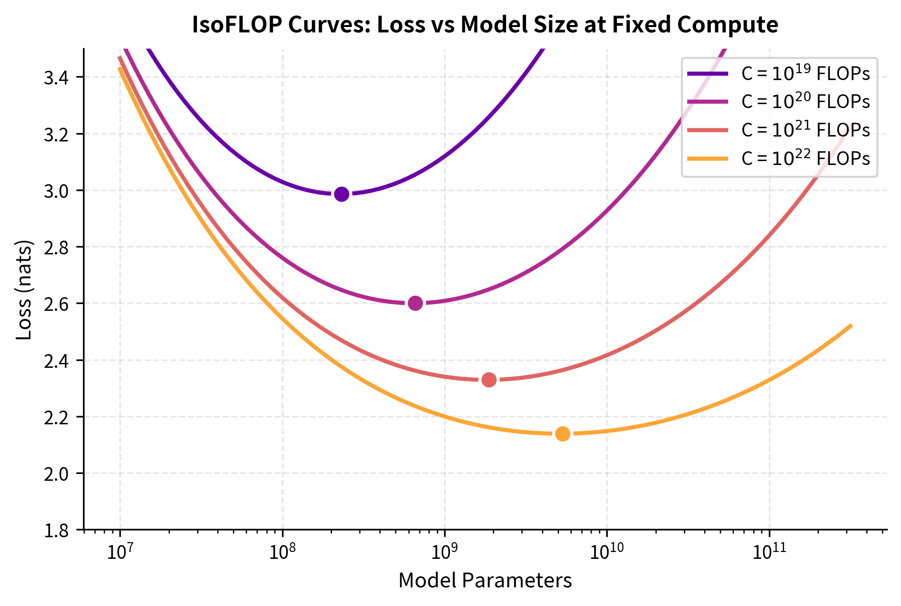
This figure from the Chinchilla paper shows several iso-FLOP curves, each corresponding to a fixed compute budget (the different colored lines). Notice how each curve has a clear minimum, representing the optimal model size for that budget. Deviating in either direction—making the model too small or too large—results in a higher loss.

This "U" shape represents two suboptimal regimes:

• Under-parameterized (Left side of the U): A model that is too small for the compute budget. It is trained on a massive amount of data, but it lacks the capacity (parameters) to learn all the complex patterns present. You are wasting compute on redundant training signals the model cannot absorb.
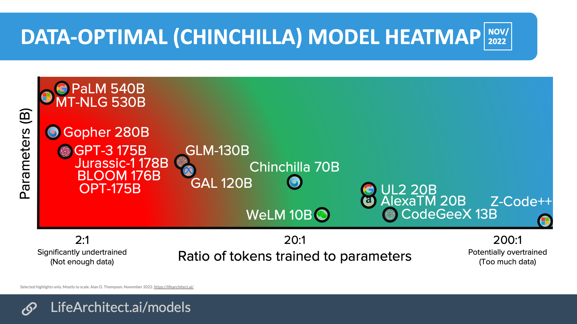
• Undertrained (Right side of the U): A model that is too large for the compute budget. It has immense capacity, but it is trained on too few tokens to learn effectively. This is where models like GPT-3 and Gopher were situated, according to the Chinchilla findings.

The bottom of the "U" is the compute-optimal point, where the balance between model capacity and training data is just right, yielding the lowest possible loss for that budget.

The following video provides an excellent summary of the three methods used in the Chinchilla paper to pinpoint this optimal balance. As you watch, focus on the logic behind each approach and how they converge on the same conclusion.

A Deeper Reconciliation: Total vs. Non-Embedding Parameters

The previous lesson mentioned differences in learning rate schedules as one reason for the discrepancy between Kaplan and Chinchilla's findings. However, a more recent paper has uncovered a subtler and more profound reason that goes to the heart of the measurement methodology. This will appeal to your interest in theoretical foundations.

The key insight, detailed in "Reconciling Kaplan and Chinchilla Scaling Laws" by Pearce and Song (2024), is that the two studies were measuring different things.

• Chinchilla counted total parameters ($N_T$), which includes all weights in the model.
• Kaplan counted non-embedding parameters ($N_{\backslash E}$), excluding the large token and positional embedding layers.

Why does this matter? The number of embedding parameters ($N_E$) is determined by the vocabulary size ($v$) and the model dimension ($d$), i.e., $N_E\approx v\times d$. For smaller models, the embedding layer can constitute a very large fraction of the total parameters. As models get bigger, this fraction shrinks, and $N_T$ becomes approximately equal to $N_{\backslash E}$.

This creates a non-linear relationship between $N_T$ and $N_{\backslash E}$, especially at the smaller model sizes that Kaplan's analysis focused on. Pearce and Song demonstrated that this seemingly minor methodological choice was the primary cause of the different scaling exponents. When they re-analyzed the Chinchilla data using Kaplan's approach—counting non-embedding parameters and focusing on smaller models—they were able to reproduce Kaplan's original scaling exponent of $N_{\text{opt}}\propto C^{0.73}$!

This shows that Kaplan's finding wasn't necessarily "wrong," but rather a "local" power law that holds true under a specific set of measurement assumptions. The Chinchilla law, using total parameters, proved to be more general and robust across scales.

To get the authors' own summary of this elegant piece of scientific detective work, please read the opening of their paper.

From Theory to Practice: Budgeting your FLOPs

Now, let's make this concrete. How do you use the Chinchilla laws to plan a training run? Assume you are given a compute budget $C$ and need to determine the optimal model size $N$ and number of training tokens $D$.

We have two key equations:

1. The compute approximation: $C\approx 6ND$
2. The Chinchilla ratio: $D/N\approx 20$

By substituting the second equation into the first, we can solve for the optimal model size, $N_{\text{opt}}$, as a function of only the compute budget $C$:
$C\approx 6N(20N)=120N^2$
$N_{\text{opt}}\approx \sqrt{\frac{C}{120}}$

Once you have $N_{\text{opt}}$, you can easily find the optimal number of tokens:
$D_{\text{opt}}\approx 20\times N_{\text{opt}}$

This simple set of equations forms a powerful tool for resource planning. To see this in action, the following article provides a superb step-by-step example and even provides Python code to implement the calculation, which should resonate well with your hands-on background.

Beyond Training Optimality: Inference and Data Constraints

The Chinchilla laws are designed to find the model that achieves the lowest loss for a given training compute budget. However, in any real-world deployment, other factors come into play.

1. Inference Costs

As a DevOps lead, you know that training is often a one-time capital expenditure, while inference is an ongoing operational cost. For a widely used product, inference costs will quickly dwarf the initial training cost.

Here, the Chinchilla approach provides a double benefit. A smaller, Chinchilla-optimal model (e.g., 70B parameters) is not only better-performing than a larger, undertrained one (e.g., 280B parameters), but it's also dramatically cheaper to run at inference time. The memory footprint is smaller, and the number of operations per generated token is lower. This has led to a modern focus on inference-optimal scaling, which may favor even smaller models trained on even more data than the Chinchilla prescription.

2. Data Constraints: Hitting the "Data Wall"

The Chinchilla framework implicitly assumes you have access to a virtually unlimited supply of high-quality training data. But what happens when that's no longer true? A 1 trillion parameter model, according to the 20:1 rule, would require 20 trillion tokens of unique, high-quality text. The entire public web is estimated to contain between 50 and 100 trillion tokens, much of it low-quality.

We are approaching a "data wall," where data, not compute, becomes the primary bottleneck. This introduces a new set of tradeoffs and has spurred research into:

• Synthetic data generation: Using models to create new training data.
• Multi-epoch training: Training on the same data more than once, though this yields diminishing returns.
• Aggressive data curation: Focusing on extremely high-quality data subsets.

The Stanford lecture briefly touches on this evolving perspective.

Conclusion

In this lesson, we have moved from simply knowing the scaling laws to actively analyzing the tradeoffs they represent. By understanding how to balance model size and dataset size for a fixed compute budget, you are now equipped with the fundamental strategic framework used by every major AI lab.

Here are the key takeaways from our analysis:

• The U-Shaped Tradeoff: For any fixed compute budget, there is an optimal allocation of resources. Models that are too small (under-parameterized) or too large (undertrained) will perform suboptimally.
• Reconciliation through Methodology: The apparent conflict between Kaplan and Chinchilla's findings was largely resolved by understanding a key methodological difference: counting total versus non-embedding parameters.
• A Practical Formula: The Chinchilla laws provide a concrete recipe for budget allocation: $N_{\text{opt}}\approx \sqrt{C/120}$ and $D_{\text{opt}}\approx 20\times N_{\text{opt}}$.
• Real-World Constraints: While powerful, these laws focus on training compute. Practical decisions must also weigh inference costs and the finite availability of high-quality data, which are pushing the field toward even more data-intensive training regimes.

So far, our discussion of scaling has been purely quantitative—more compute, more parameters, more data lead to a lower loss. But what happens to the behavior of the model as it scales? In our next lesson, we will explore the fascinating phenomenon of emergent capabilities, where quantitative increases in scale lead to surprising, qualitative leaps in what models can do.