Chinchilla Scaling Laws: Revising Compute-Optimal Allocation

A New Rule for Scaling: Balance is Key

The central finding of the Chinchilla paper is a direct rebuttal to the "model size first" approach. The DeepMind team found that for optimal performance, model size and the number of training tokens should be scaled in equal proportion.

Recall Kaplan's allocation:

• Optimal Model Size: $N_{\text{opt}}\propto C^{0.73}$
• Optimal Dataset Size: $D_{\text{opt}}\propto C^{0.27}$

The Chinchilla paper proposed a revised set of exponents:

• Optimal Model Size: $N_{\text{opt}}\propto C^{0.5}$
• Optimal Dataset Size: $D_{\text{opt}}\propto C^{0.5}$

This seemingly small change in exponents has enormous practical consequences. It implies that if you have 100 times more compute, you shouldn't build a model that's ~50 times bigger trained on ~2 times more data (Kaplan's advice). Instead, you should build a model that's 10 times bigger and train it on 10 times more data.

This led to the famous "Chinchilla rule": for compute-optimal training, a model should be trained on approximately 20 tokens for every parameter it has.

To begin, let's go directly to the source. The abstract and introduction of the paper provide a concise summary of this core argument.

Why the Discrepancy? Revisiting the Methodology

How could two different research groups, both conducting extensive experiments, arrive at such different conclusions? The answer lies in subtle but critical differences in experimental methodology. A key issue identified by the DeepMind team was the handling of the learning rate schedule.

As we discussed in the pre-training module, a common strategy is to use a learning rate that warms up and then decays over the course of training (e.g., a cosine schedule). The Kaplan et al. experiments used a fixed schedule length for all models. This meant that models trained on more data (i.e., for more steps) would have their learning rate decay to its minimum value relatively early, and then continue training with a tiny, ineffective learning rate for the remainder of the run. This systematically underestimated the benefit of training for longer on more data.

Professor Mohit Iyyer from UMass provides a succinct explanation of this issue.

The authors of the Chinchilla paper explicitly addressed this limitation. By carefully tailoring the learning rate schedule to match the number of training tokens for each run, they were able to get a much more accurate signal about the true value of additional data.

Three Paths to the Same Conclusion

The strength of the Chinchilla paper lies in its rigorous methodology. Instead of relying on a single method, the researchers used three distinct approaches to estimate the optimal scaling law. The fact that all three converged on a similar result provides strong evidence for their conclusion.

Here's a brief overview of the three approaches:

1. Approach 1: Fixed Model Sizes. The team trained models of several fixed sizes (e.g., 70M, 1B, 10B parameters) and varied the number of training tokens for each. By plotting the loss curves, they could find the "lower envelope"—the optimal performance achievable for any given FLOPs budget—and deduce the model size and token count that achieved it.

2. Approach 2: IsoFLOP Curves. The team fixed several total compute budgets (e.g., $10^{19}$ FLOPs, $10^{20}$ FLOPs). For each budget, they trained various models, trading off parameters for tokens (e.g., a big model on few tokens vs. a small model on many tokens). Plotting loss against model size for a fixed budget results in a U-shaped "iso-FLOP" curve. The minimum of this curve reveals the optimal model size for that specific budget.

3. Approach 3: Parametric Loss Fitting. This approach models the final loss as a parametric function of model size ($N$) and dataset size ($D$). The function they proposed is:
   $L(N,D)\approx E+\frac{A}{N^{\alpha }}+\frac{B}{D^{\beta }}$
   Here, $E$ represents the irreducible loss (the entropy of language), the $A/N^{\alpha }$ term represents the error from finite model size, and the $B/D^{\beta }$ term represents the error from a finite number of training tokens. By training over 400 models with different $N$ and $D$ and fitting this function, they could solve for the optimal allocation mathematically.

The following segment from the Stanford lecture on scaling laws provides an excellent, detailed walkthrough of these three methods.

As the lecturer notes, there was a fascinating follow-up story where other researchers discovered a minor curve-fitting error in Approach 3. When corrected, the result from Approach 3 aligned even more perfectly with the other two, strengthening the paper's overall conclusion.

The Proof: Chinchilla vs. Gopher

Armed with their new scaling laws, the DeepMind team put their hypothesis to the test. At the time, DeepMind's flagship model was Gopher, a 280B parameter model trained on 300B tokens, following the Kaplan-style philosophy.

The new scaling law predicted that for the same compute budget used to train Gopher, a much smaller model trained on far more data would be optimal. They designed Chinchilla: a 70B parameter model (4x smaller than Gopher) trained on 1.4 trillion tokens (~4.5x more data).

The result was a resounding success. Despite being significantly smaller, Chinchilla outperformed Gopher, GPT-3 (175B), and other larger models on a wide range of downstream tasks. This was concrete proof that the compute-optimal strategy had shifted.

The following article provides a clear, practical breakdown of the final equations and includes a worked example that makes the abstract formulas concrete—something that should resonate with your technical background.

The Impact on the Field

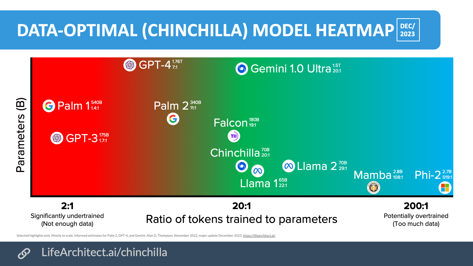
The Chinchilla paper had an immediate and lasting impact. It became clear that many of the largest models were sitting in the "undertrained" region—they were too large for the amount of data they had seen. Subsequent major models, like Meta's Llama series, adopted the Chinchilla philosophy, opting for smaller parameter counts (e.g., 7B to 70B) but training them on trillions of tokens.

This heatmap vividly illustrates the shift. Models in the red zone are undertrained (too few tokens per parameter), while models in the green zone are closer to the compute-optimal Chinchilla ratio.

Conclusion

In this lesson, we've traced the evolution of scaling laws from the initial findings of Kaplan et al. to the crucial revisions introduced by the Chinchilla paper. This journey highlights the self-correcting nature of the scientific process and provides a deeper, more nuanced understanding of the resources required to build powerful language models.

Here are the key takeaways:

• Revised Allocation: The Chinchilla scaling laws revised the compute-optimal strategy, showing that model size and dataset size should be scaled equally ($N\propto C^{0.5},D\propto C^{0.5}$).
• The 20:1 Rule: This leads to a practical rule of thumb: for compute-optimal training, a model should see approximately 20 tokens per parameter.
• Methodological Rigor: The conclusion was supported by three independent experimental methods and confirmed by training Chinchilla (70B), which outperformed the much larger Gopher (280B) model using the same compute budget.
• Paradigm Shift: The findings revealed that previous large models like GPT-3 were significantly undertrained. This shifted the industry's focus from a pure race for parameter count to a more balanced approach that heavily emphasizes the quantity and quality of training data.

We have now established a robust quantitative framework for thinking about scale. But what happens at that scale? It turns out that simply making models bigger doesn't just lead to better performance on existing tasks; it can lead to entirely new, unpredicted behaviors. In our next lesson, we will explore these fascinating emergent capabilities, such as in-context learning, and discuss the idea that for LLMs, "more is different."