Understanding Friction: Opposing Motion

Part 1: The Physics of Friction

Before we write any code, let's establish a solid understanding of the physics. Friction is a force that resists the relative motion—or tendency of such motion—between surfaces in contact.

To get a clear overview, let's start with a short video that explains the fundamentals.

As the video explained, there are two main types of friction we need to consider:

• Static Friction ($F_s$): This is the "gripping" force. It acts on an object at rest and prevents it from moving. It has a maximum value. If the force trying to move the object is less than this maximum, the object stays put.
• Kinetic Friction ($F_k$): This is the "sliding" force. It acts on an object that is already in motion. It has a constant value and is typically less than the maximum static friction. This is why it's often harder to get a heavy box moving than to keep it sliding.

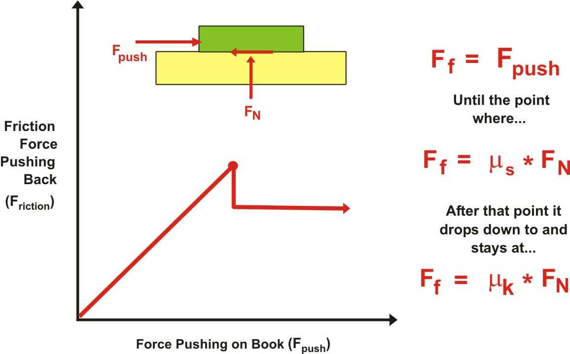
The magnitude of the friction force is proportional to the normal force ($N$), which is the force pressing the two surfaces together. In our collision system, the impulse we calculated in the last lesson to make objects bounce apart is directly related to this normal force. This is a key connection we will leverage.

Part 2: Modeling Friction as an Impulse

In our engine, we handle collision responses with instantaneous changes in velocity, called impulses. The "bounce" impulse from the last lesson was applied along the collision normal to push the objects apart.

Friction, which resists sliding, acts perpendicular to the collision normal, along the plane of contact. Therefore, we can model friction as a second impulse, the friction impulse, applied along the tangent of the collision surface.

The following video provides an excellent, detailed walkthrough of this exact technique. It will be the primary guide for our implementation.

Once we have the normalized tangent vector $\mathbf{t}$, we can calculate the friction impulse required to stop this sliding motion. The calculation is analogous to how we found the normal impulse $j$ in the last lesson, but we use $\mathbf{t}$ instead of $\mathbf{n}$.

Part 3: Coulomb's Law and Clamping the Impulse

As we know from the physics, friction isn't limitless. The friction impulse can't be stronger than what the normal force allows. This physical constraint is described by Coulomb's Law of Friction. In our impulse-based model, this translates to:

The magnitude of the friction impulse, ${\mathbf{j}}_{\mathbf{t}}$, must be less than or equal to the magnitude of the normal impulse, $\mathbf{j}$, multiplied by the coefficient of static friction, ${\mu }_s$.
$|{\mathbf{j}}_{\mathbf{t}}|\le |\mathbf{j}|\cdot {\mu }_s$

This gives us the logic for our collision response:

1. Calculate the potential friction impulse ${\mathbf{j}}_{\mathbf{t}}$ needed to completely stop the sliding.
2. Check if its magnitude is less than $|\mathbf{j}|\cdot {\mu }_s$.
   • If it is (static friction holds): The final friction impulse is ${\mathbf{j}}_{\mathbf{t}}$. The sliding motion is stopped.
   • If it isn't (static friction breaks): The object starts sliding. The friction impulse is clamped to a smaller magnitude, determined by the kinetic friction coefficient: $|\mathbf{j}|\cdot {\mu }_k$.

This process is explained very clearly in the next part of the video.

Part 4: Implementation in C

Now, let's integrate this into our project. We'll modify the PhysicsBody struct and the resolve_sphere_collision function from the previous lesson.

1. Update the PhysicsBody Struct

First, add friction coefficients to PhysicsBody. We'll use two: one for static friction and one for kinetic.

// In your physics component header (e.g., physics_component.h)
typedef struct {
    vec3 velocity;
    vec3 force_accumulator;
    float mass;
    float inverse_mass;
    float radius;
    float restitution;
    float static_friction;  // New!
    float dynamic_friction; // New! (Also called kinetic friction)
} PhysicsBody;

When you create your entities, you can set these values. Good defaults might be static_friction = 0.6 and dynamic_friction = 0.4. Remember, dynamic friction should generally be less than or equal to static friction.

2. Update resolve_sphere_collision

Here is the updated function. It builds directly on the code from the previous lesson, adding the logic for the friction impulse after the normal impulse has been calculated and applied.

void resolve_sphere_collision(
    Transform* t1, PhysicsBody* p1, 
    Transform* t2, PhysicsBody* p2) 
{
    // --- (Steps 1 & 2 from previous lesson are unchanged) ---
    vec3 collision_vec;
    glm_vec3_sub(t2->position, t1->position, collision_vec);

    float distance = glm_vec3_norm(collision_vec);
    float radii_sum = p1->radius + p2->radius;

    if (distance > radii_sum) {
        return; // No collision
    }

    vec3 normal;
    glm_vec3_normalize_to(collision_vec, normal);

    // --- (Step 3 from previous lesson is unchanged) ---
    vec3 relative_velocity;
    glm_vec3_sub(p2->velocity, p1->velocity, relative_velocity);
    float vel_along_normal = glm_vec3_dot(relative_velocity, normal);

    if (vel_along_normal > 0) {
        return; // Objects are already separating
    }

    // --- (Steps 4 & 5 from previous lesson - Calculate Normal Impulse) ---
    float e = fminf(p1->restitution, p2->restitution);
    float j = -(1 + e) * vel_along_normal;
    j /= p1->inverse_mass + p2->inverse_mass;

    // --- (Step 6 from previous lesson - Apply Normal Impulse) ---
    vec3 impulse_normal;
    glm_vec3_scale(normal, j, impulse_normal);

    vec3 v1_change;
    glm_vec3_scale(impulse_normal, p1->inverse_mass, v1_change);
    glm_vec3_sub(p1->velocity, v1_change, p1->velocity);

    vec3 v2_change;
    glm_vec3_scale(impulse_normal, p2->inverse_mass, v2_change);
    glm_vec3_add(p2->velocity, v2_change, p2->velocity);

    // ==========================================================
    // --- NEW: FRICTION IMPULSE CALCULATION ---
    // ==========================================================

    // 1. Recalculate relative velocity post-normal-impulse
    glm_vec3_sub(p2->velocity, p1->velocity, relative_velocity);
    
    // 2. Calculate the tangent vector
    vec3 tangent;
    float vel_dot_normal = glm_vec3_dot(relative_velocity, normal);
    vec3 vel_proj_normal;
    glm_vec3_scale(normal, vel_dot_normal, vel_proj_normal);
    glm_vec3_sub(relative_velocity, vel_proj_normal, tangent);

    if (glm_vec3_norm_squared(tangent) < 0.0001f) { // Avoid normalizing a zero vector
         // If there's no tangent velocity, there's no friction to apply.
         // We can do positional correction and then exit.
    } else {
        glm_vec3_normalize(tangent);

        // 3. Calculate magnitude of impulse required to stop sliding
        float jt = -glm_vec3_dot(relative_velocity, tangent);
        jt /= p1->inverse_mass + p2->inverse_mass;

        // 4. Get combined friction coefficients
        float static_friction = (p1->static_friction + p2->static_friction) * 0.5f;
        float dynamic_friction = (p1->dynamic_friction + p2->dynamic_friction) * 0.5f;

        // 5. Apply Coulomb's Law
        vec3 friction_impulse;
        if (fabsf(jt) < j * static_friction) {
            // Static friction holds
            glm_vec3_scale(tangent, jt, friction_impulse);
        } else {
            // Kinetic friction applies
            glm_vec3_scale(tangent, -j * dynamic_friction, friction_impulse);
        }

        // 6. Apply the friction impulse
        glm_vec3_scale(friction_impulse, p1->inverse_mass, v1_change);
        glm_vec3_sub(p1->velocity, v1_change, p1->velocity);

        glm_vec3_scale(friction_impulse, p2->inverse_mass, v2_change);
        glm_vec3_add(p2->velocity, v2_change, p2->velocity);
    }
    
    // --- (Step 7 from previous lesson is unchanged - Positional Correction) ---
    const float percent = 0.4f; // Can be a bit higher to feel more solid
    const float slop = 0.01f;
    
    float penetration = radii_sum - distance;
    if (penetration > slop) {
        float correction_amount = (penetration - slop) / (p1->inverse_mass + p2->inverse_mass) * percent;
        vec3 correction_vec;
        glm_vec3_scale(normal, correction_amount, correction_vec);

        vec3 t1_correction;
        glm_vec3_scale(correction_vec, p1->inverse_mass, t1_correction);
        glm_vec3_sub(t1->position, t1_correction, t1->position);

        vec3 t2_correction;
        glm_vec3_scale(correction_vec, p2->inverse_mass, t2_correction);
        glm_vec3_add(t2->position, t2_correction, t2->position);
    }
}

Update your physics_system_update loop to call this new function. The loop itself doesn't need to change from the last lesson. When you run your simulation, you should now see objects realistically slow down as they rub against each other and come to a stop.

Conclusion

Congratulations on implementing friction! This is a significant step that adds a great deal of nuance and realism to your physics engine. The objects in your world no longer feel like they're weightless pucks on an air hockey table.

Key Takeaways:

• Friction is a force that opposes relative motion and can be modeled as static (gripping) and kinetic/dynamic (sliding).
• In an impulse-based physics system, friction can be implemented as an impulse applied along the tangent of the collision surface, perpendicular to the normal.
• Coulomb's Law provides the critical constraint: the friction impulse's magnitude is limited by the normal impulse. This allows us to determine whether static friction holds or kinetic friction takes over.
• The implementation builds directly on our previous collision response system by adding a second impulse calculation after the normal (bounce) impulse is resolved.

Preview of the Next Lesson:
Our physics simulation is now quite sophisticated. We've covered forces, collision detection, and responses including bounces and friction. It's time to shift our focus to another critical component of any game: audio. In the next lesson, we will begin the "Audio Integration" module by learning how to set up an audio library like miniaudio in our C project, laying the groundwork for adding sound effects and music to our game world.