Analyzing Onset and Overpotential from LSV Curves

The Prerequisite: iR Correction

Before we can accurately determine any kinetic parameters from a polarization curve, we must first account for an experimental artifact known as the ohmic drop, or $iR$ drop. This is a voltage loss that occurs due to the inherent resistance ($R_s$) of the electrolyte, electrical contacts, and the electrode material itself. This resistance causes a potential drop, $\Delta E=i{R}_s$, which is purely a function of the system's resistance and the current flowing through it.

This ohmic potential loss is not related to the catalytic activity at the electrode-electrolyte interface. It's an instrumental artifact that "stretches" the polarization curve along the potential axis, making the catalyst appear less active than it truly is. To evaluate the intrinsic kinetics of your catalyst, you must correct for it.

The standard procedure for iR correction involves subtracting the ohmic drop from the measured potential at each point.

As you've just read, the corrected potential ($V_{\text{corrected}}$) is calculated as:

Often, a partial correction (80-100%) is applied to avoid overcorrection, as noted in the resource which suggests using $0.9\times R_s$. The solution resistance, $R_s$, is typically measured using Electrochemical Impedance Spectroscopy (EIS), a topic we will cover in detail in Module 6. For now, it is crucial to understand that this correction is the mandatory first step in your data analysis workflow. All subsequent parameters must be extracted from the iR-corrected curve.

Determining the Onset Potential ($E_{\text{onset}}$)

The onset potential marks the point at which the catalytic reaction "turns on" and a significant Faradaic current begins to flow. Conceptually, a catalyst with an onset potential closer to the thermodynamic equilibrium potential is more active, as it requires less of an energetic push to initiate the reaction. There are a few methods to determine it.

1. The Threshold Current Density Method

This is the most objective and widely adopted method in recent literature. It defines the onset potential as the potential required to reach a small, pre-defined "threshold" current density. This removes the ambiguity of visual interpretation. For HER and OER, this threshold is often set to a value like 1 mA/cm², 0.5 mA/cm², or even lower.

As the protocol suggests, a value like -0.1 mA/cm² can be used for HER. The key is to be consistent and to always report the threshold value you used. This requires you to first convert your measured current ($I$, in Amperes) to current density ($j$, in A/cm²) by dividing by the geometric surface area of your electrode. We will explore this normalization in more detail in the next lesson.

2. The Tangent Intersection Method

A more traditional, graphical method involves drawing two tangent lines on the polarization curve:

• One tangent along the non-Faradaic baseline where only capacitive current is present.
• A second tangent along the steeply rising part of the curve where the catalytic current dominates.

The potential at which these two lines intersect is defined as the onset potential.

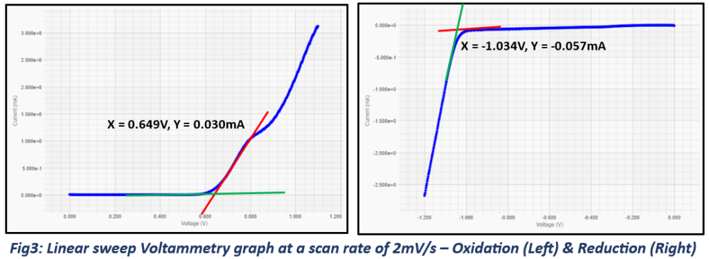
While visually intuitive, this method can be subjective as the placement of the tangent on the exponential part of the curve can vary between analyses.

3. The Second Derivative Method

For a more mathematically rigorous determination, one can analyze the derivatives of the LSV curve. The onset of a new electrochemical process corresponds to a change in the slope of the curve. The potential at which the second derivative of the current with respect to potential (d²I/dV²) reaches a minimum can be defined as the onset potential.

Given your experience with data analysis in OriginPro, you could implement such a derivative analysis for high-precision work. However, for most reporting, the threshold current density method is the preferred standard.

Determining Overpotential at a Benchmark Current Density (${\eta }_j$)

While the onset potential tells us when the reaction starts, the overpotential tells us how much extra voltage is needed to drive the reaction at a specific, meaningful rate. This is arguably the most important metric for comparing catalyst efficiency. This rate is defined by a benchmark current density ($j$), typically 10 mA/cm² for lab-scale catalyst screening. This value is relevant because it approximates the current density that would be produced by a 1-sun solar-to-fuel device.

The calculation follows these steps:

1. Start with your iR-corrected LSV data.

2. Normalize your current to current density ($j$).

3. Find the potential ($E_j$) on your polarization curve that corresponds to the benchmark current density (e.g., $j$ = 10 mA/cm² or 0.01 A/cm²). You can do this easily in a program like OriginPro by interpolating your data.

4. Calculate the overpotential ($\eta$) by subtracting the thermodynamic equilibrium potential ($E_{\text{eq}}$) from your measured potential $E_j$.

   $${\eta }_j=E_j-E_{\text{eq}}$$

   Recall from Module 1 that for reactions referenced to the Reversible Hydrogen Electrode (RHE) scale:

   • HER: $E_{\text{eq}}=0.0$ V vs. RHE
   • OER: $E_{\text{eq}}=1.23$ V vs. RHE

The following video provides a practical walkthrough of this exact process for an OER catalyst using data analysis software.

As the video and the CEN protocol highlight, a lower overpotential at the benchmark current density signifies a more energy-efficient catalyst, which is the primary goal of your research. While 10 mA/cm² is a standard for comparison, for practical electrolyser applications, performance at much higher current densities (e.g., 200, 500, or even 1000 mA/cm²) is what truly matters, as this dictates the hydrogen production rate of a device.

To see how these metrics are used in a real research context, the following presentation provides excellent examples.

Conclusion

In this lesson, you have learned the systematic process for analyzing LSV polarization curves to extract meaningful performance metrics. This is the bridge between collecting electrochemical data and drawing conclusions about your catalyst's efficacy.

Key Takeaways:

• iR correction is a mandatory first step in LSV data analysis to remove ohmic artifacts and evaluate the catalyst's true kinetic performance. The corrected potential is given by $V_{\text{corrected}}=V_{\text{measured}}-I\times R_s$.
• The onset potential ($E_{\text{onset}}$) indicates the potential at which the reaction begins. The most objective method for its determination is finding the potential that corresponds to a small, defined threshold current density (e.g., 1 mA/cm²).
• The overpotential at a benchmark current density (${\eta }_j$) is a key measure of catalyst efficiency. It is calculated as ${\eta }_j=E_j-E_{\text{eq}}$, where $E_j$ is the iR-corrected potential required to reach a benchmark like 10 mA/cm².
• A lower onset potential and a lower overpotential signify a more active and energy-efficient electrocatalyst.

Preview of the Next Lesson:

We have repeatedly mentioned the need to convert raw current into current density by normalizing to the electrode's area. In the next lesson, we will dedicate our full attention to this crucial step. We will discuss normalization by geometric area, how to use the ECSA you learned to calculate in Lesson 5.3 to determine intrinsic activity, and normalization by catalyst mass. This will complete your toolkit for rigorously reporting and comparing electrocatalytic performance.