Choosing the Right Ensemble: Constraints and Convenience

Welcome back. In our previous lesson, we completed a significant milestone by deriving the Sackur-Tetrode equation for the entropy of an ideal gas. This was not merely an exercise; it resolved the Gibbs paradox by demonstrating the crucial role of particle indistinguishability and the $1/ N!$ correction, which ensures entropy is properly extensive. This calculation, performed within the microcanonical ensemble, also underscored a key challenge: counting states under a strict energy constraint can be mathematically demanding.

Building on that experience, we now turn to a more strategic and practical question. Our goal for this lesson is to justify the choice of a specific ensemble (microcanonical, canonical, or grand canonical) for solving a given physical problem based on constraints and computational convenience. While we've established that these ensembles are equivalent for calculating thermodynamic averages in the large-system limit, the ease and feasibility of the calculation can differ dramatically. Understanding these differences is essential for a practicing physicist.

1. The Ensembles: A Conceptual and Physical Overview

At its heart, an ensemble is a collection of all possible microstates a system can be in, consistent with a given set of macroscopic constraints. The choice of ensemble is therefore a choice of which macroscopic quantities we consider fixed. The three principal ensembles in statistical mechanics correspond to three common physical situations.

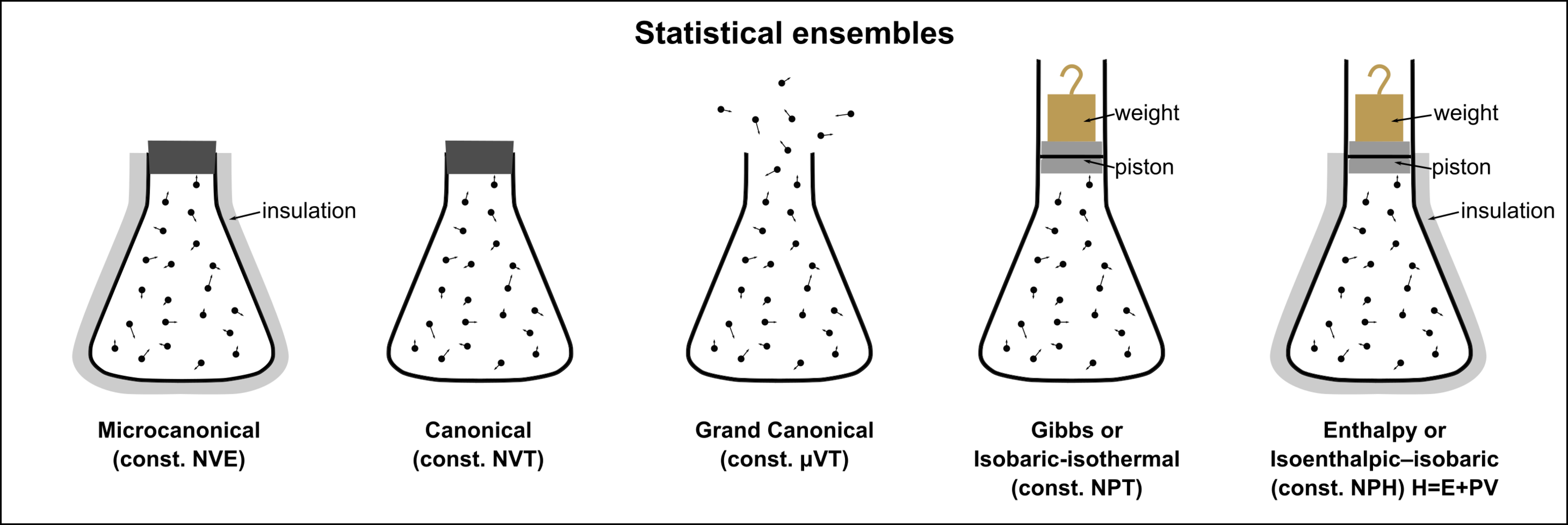
This image illustrates the different boundary conditions for the microcanonical, canonical, grand canonical, and other ensembles. The type of wall (insulating, diathermal, permeable) determines what can be exchanged with the surroundings.

Let's formalize the distinctions using the lecture notes from Matthew Schwartz at Harvard.

Lecture 7: Ensembles

These notes provide a concise introduction to the main statistical ensembles, defining their fixed properties and the key computational objects associated with each.

Please read the introduction (Section 1) and the summary (Section 9) to get a clear, comparative overview of the microcanonical, canonical, and grand canonical ensembles. Focus on the table of conjugate pairs (E, T), (N, μ), (V, P) and which variable is fixed in each ensemble.

As the notes and the image above clarify:

Microcanonical Ensemble (NVE): This describes a completely isolated system. The number of particles $N$ , volume $V$ , and total energy $E$ are all strictly fixed. No energy or matter can be exchanged with the surroundings. This is the most fundamental ensemble, as it relies directly on the postulate of equal a priori probabilities. The central quantity to compute is the number of accessible microstates, $Ω (N, V, E)$ , from which we derive the entropy $S = k_{B} ln Ω$ .
Canonical Ensemble (NVT): This describes a closed system in thermal contact with a heat reservoir at a fixed temperature $T$ . The system can exchange energy with the reservoir, so its own energy $E$ fluctuates. $N$ and $V$ remain fixed. This is an excellent model for many laboratory experiments, where a sample is held at a constant temperature. The central quantity is the canonical partition function, $Z (N, V, T) = \sum_{k} e^{- β E_{k}}$ .
Grand Canonical Ensemble ( $μ$ VT): This describes an open system that can exchange both energy and particles with a large reservoir. The system's energy $E$ and particle number $N$ both fluctuate. The system is characterized by a fixed chemical potential $μ$ , volume $V$ , and temperature $T$ . This is the natural ensemble for systems involving chemical reactions or phase equilibria, where particle numbers are not constant. The key quantity is the grand partition function, $Ξ (μ, V, T) = \sum_{k} e^{- β E_{k} + β μ N_{k}}$ .

The following video provides an excellent summary of this hierarchy and the physical reasoning behind each ensemble.

15. Interacting Particles Part 1

This MIT OpenCourseWare lecture by Prof. Mehran Kardar provides a clear walkthrough of the rationale behind the different ensembles.

Please watch the following segments: A review of the microcanonical ensemble here. The motivation and setup for the canonical ensemble here. The motivation and setup for the Gibbs (isobaric-isothermal) ensemble, which fixes P instead of V, here. This is a close relative of the canonical ensemble. The motivation and setup for the grand canonical ensemble here.

2. The Trade-off: Foundational Purity vs. Computational Convenience

If all ensembles are equivalent in the thermodynamic limit, why not always use the most fundamental one, the microcanonical ensemble? The answer, as you might have suspected from our derivation of the Sackur-Tetrode equation, is computational difficulty.

The Microcanonical Challenge: The Tyranny of the Constraint

Calculating $Ω (N, V, E)$ requires counting states on a constant-energy surface in a $6 N$ -dimensional phase space.
$E = \sum_{i = 1}^{N} \frac{p _{i}^{2}}{2 m} + U (q_{1}, \dots, q_{N})$
For the ideal gas, $U = 0$ , so this constraint defines a hypersphere in momentum space. The calculation was non-trivial but feasible. For an interacting system ( $U \neq = 0$ ), the constraint couples all position and momentum coordinates in a complex way. The constant-energy surface is no longer a simple geometric object, and calculating its "area" is often intractable. The core problem is the strict energy constraint, which manifests as a difficult, constrained sum or integral.

The Canonical Solution: The Power of the Unconstrained Sum

The canonical ensemble circumvents this difficulty. The partition function $Z = \sum_{k} e^{- β E_{k}}$ is a sum over all possible microstates, regardless of their energy, weighted by the Boltzmann factor. This unconstrained sum is mathematically far more tractable.

Consider an interacting classical gas again. The partition function is:
$Z = \frac{1}{N ! h ^{3 N}} \int e^{- β (\sum_{i} \frac{p _{i}^{2}}{2 m} + U (q))} d^{3 N} p d^{3 N} q$
Crucially, the exponential of a sum is a product of exponentials. The integral separates into a kinetic part and a potential part:
$Z = \frac{1}{N ! h ^{3 N}} (\int e^{- β \sum_{i} \frac{p _{i}^{2}}{2 m}} d^{3 N} p) (\int e^{- β U (q)} d^{3 N} q)$
The momentum integral is just a product of $3 N$ independent Gaussian integrals, identical to the ideal gas case! All the difficulty of the interactions is isolated in the configurational integral, $\int e^{- β U (q)} d^{3 N} q$ . While this integral is still very difficult, it is an unconstrained integral and forms the starting point for many powerful approximation techniques (like perturbation theory, which you may have encountered in quantum mechanics).

The following video segment lucidly explains this advantage.

15. Interacting Particles Part 1

Prof. Kardar explains why calculating properties of interacting systems is often much more feasible in the canonical ensemble.

Watch the segment from this point, where he sets up the canonical partition function for an interacting gas and shows how the momentum and coordinate integrals separate, isolating the difficult part into a more manageable form compared to the microcanonical approach.

The grand canonical ensemble offers even greater convenience in certain cases, particularly for non-interacting quantum particles. By allowing the particle number $N$ to vary, the grand partition function $Ξ$ can often be factorized into a product over single-particle energy states. This incredible simplification is the reason we will use the grand canonical ensemble almost exclusively when deriving the Fermi-Dirac and Bose-Einstein distributions in a later module.

3. A Practical Guide to Choosing Your Ensemble

With this understanding of the physical basis and computational trade-offs, we can formulate a practical guide.

Ensemble	Fixed Quantities	Physical System	When to Use It
Microcanonical	$N, V, E$	Perfectly isolated system.	Theoretical Foundations: For deriving fundamental results from first principles (e.g., Boltzmann entropy). Specialized Systems: Small, isolated systems (nuclei, star clusters) or systems with long-range interactions where ensembles may not be equivalent.
Canonical	$N, V, T$	Closed system in a heat bath.	The Workhorse: The default choice for most macroscopic systems where temperature is controlled and particle number is fixed. Computationally much easier than the microcanonical ensemble.
Grand Canonical	$μ, V, T$	Open system, exchanging energy and particles with a reservoir.	Variable Particle Number: Systems with chemical reactions or adsorption. Quantum Statistics: Indispensable for deriving properties of quantum gases (fermions, bosons, photons, phonons) where particles can be created or occupy states.

4. When the Choice Matters: Ensemble Non-Equivalence

We have operated under the assumption that for large systems, the choice of ensemble is one of convenience because the results will be the same. This is known as the equivalence of ensembles. This equivalence rests on the fact that fluctuations of thermodynamic quantities (like energy in the canonical ensemble) are vanishingly small. For instance, we've previously shown the relative energy fluctuations scale as $Δ E / ⟨ E ⟩ \propto 1/ N$ .

However, this equivalence is not universally guaranteed. Your background in advanced physics and your goal of pursuing theoretical research make this an opportune moment to introduce a deeper concept: ensemble non-equivalence. This phenomenon occurs in certain systems, most notably those with long-range interactions (like gravity) or some mean-field models.

The mathematical root of this non-equivalence lies in the properties of the microcanonical entropy $S (E)$ . For standard systems, $S (E)$ is a concave function ( $S^{''} (E) \leq 0$ ). This corresponds to a positive heat capacity, since $C_{V} = T (\partial S / \partial T)_{V}$ and $1/ T = (\partial S / \partial E)_{V}$ .

In some systems, $S (E)$ can have a non-concave region.

In this region, the heat capacity $C_{V}$ would be negative.
The canonical ensemble, whose energy fluctuations are governed by $⟨(Δ E)^{2} ⟩ = k_{B} T^{2} C_{V}$ , cannot have a negative heat capacity (since variance must be positive).
Therefore, the canonical ensemble is "blind" to these states. It cannot describe the system's behavior in that energy range. The system exhibits a first-order phase transition in the canonical ensemble, "jumping over" the thermodynamically unstable region that the microcanonical ensemble can still describe.

In such cases, the microcanonical ensemble is not just more fundamental; it is the only correct one for describing the system across all energies. The choice is no longer one of convenience, but of physical accuracy.

The document below is a PhD thesis dedicated to this very topic. While a full reading is not necessary, skimming the introductory and summary sections will give you a robust, modern perspective on this fascinating issue.

Equivalence and Nonequivalence of the Microcanonical ...

This thesis by Hugo Touchette is a landmark work connecting statistical mechanics to large deviation theory and providing a rigorous framework for understanding ensemble equivalence.

I recommend you browse the following parts to grasp the core ideas: The introduction to Chapter 2, "Statistical Mechanics as a Large Deviations Theory", to see how ensembles are formally constructed. The introduction to Chapter 3, "Equivalence and Nonequivalence", which defines equivalence based on the concavity of the entropy function. The introduction to Chapter 4, "Macrostate Level", which discusses the consequences for equilibrium states. Finally, the "Main Conclusions" section at the end for a concise, non-technical summary of the key findings.

Conclusion

In this lesson, we have moved from the abstract principle of ensemble equivalence to the practical art of ensemble choice.

Key Takeaways:

The choice of ensemble is determined by the physical constraints of the system: isolated (microcanonical), closed at fixed T (canonical), or open (grand canonical).
For most macroscopic systems with short-range interactions, the ensembles yield identical thermodynamic predictions, and the choice is dictated by computational convenience.
The canonical ensemble is generally the "workhorse" because its unconstrained sum over states is mathematically more tractable than the constrained sum of the microcanonical ensemble, especially for interacting systems.
The grand canonical ensemble offers further computational advantages for systems with fluctuating particle numbers, and is particularly crucial for quantum statistics.
Ensemble equivalence can break down, typically in systems with long-range interactions. In these cases, the microcanonical ensemble is the only one that can describe all equilibrium states, highlighting its fundamental nature beyond just being a starting point.

We have now concluded our foundational exploration of equilibrium statistical mechanics and the major ensembles. In the next module, we will pivot to apply this powerful formalism to the quantum world. We will begin by defining the quantum mechanical analogue of the classical distribution function—the density matrix—and see how our ensemble framework translates seamlessly to describe quantum systems.

Recommended resources