The Density Matrix and Von Neumann Equation

1. From State Vectors to Density Matrices

In your study of quantum mechanics, you have become accustomed to describing the state of a system with a state vector $|\psi ⟩$ residing in a Hilbert space. This description is complete; $|\psi ⟩$ contains all the information that can be known about the system. Such a state is called a pure state.

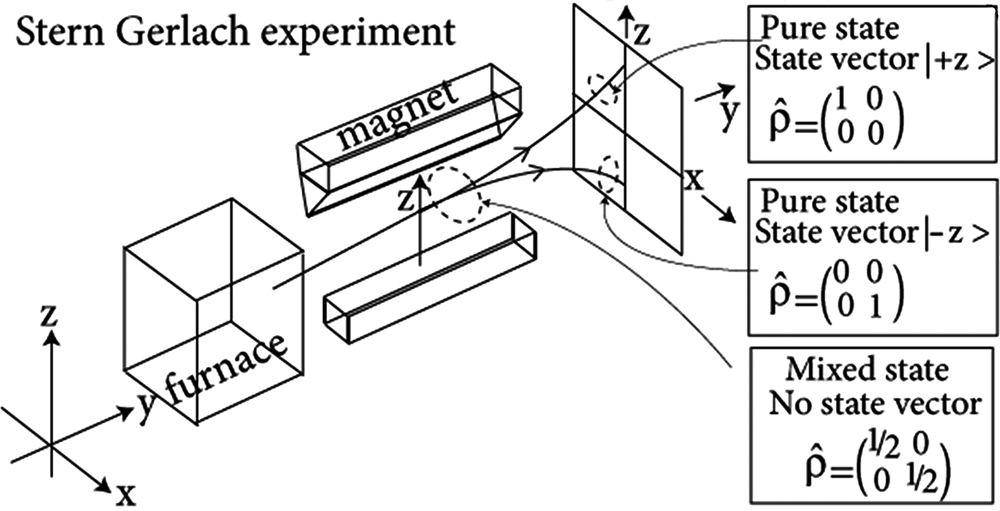
However, in statistical mechanics, we are often concerned with systems that are not in a pure state. For instance, a beam of silver atoms emerging from a furnace is not in a single quantum spin state. Instead, it's an incoherent collection of atoms, with roughly 50% in the spin-up state and 50% in the spin-down state. We don't have a single state vector for the beam; rather, we have a statistical ensemble. This is known as a mixed state.

It is crucial to distinguish a mixed state from a quantum superposition. A state like $\frac{1}{\sqrt{2}}(|\uparrow ⟩+|\downarrow ⟩)$ is a pure state, where a definite phase relationship exists between the components. A mixed state, on the other hand, represents classical uncertainty: the system is in state $|{\psi }_i⟩$ with a classical probability $p_i$, and there is no phase coherence between the different states in the ensemble.

To handle both pure and mixed states within a single mathematical framework, we introduce the density matrix, or density operator, $\hat{\rho }$.

2. The Density Operator for Pure States

Let's begin by reformulating the description of a pure state $|\psi ⟩$ using a density operator.

As you've just read, for a pure state $|\psi ⟩$, the density operator is defined as the projection operator onto that state:

The key properties that follow directly from this definition are:

1. Hermiticity: ${\hat{\rho }}^{†}=\hat{\rho }$
2. Normalization: $\text{Tr}(\hat{\rho })=1$
3. Idempotency: ${\hat{\rho }}^2=\hat{\rho }$ (as it is a projector)
4. Positivity: $\hat{\rho }$ is a positive semi-definite operator, meaning $⟨\varphi |\hat{\rho }|\varphi ⟩\ge 0$ for any state $|\varphi ⟩$.

The most important operational property is the calculation of expectation values. The standard formula $⟨A⟩=⟨\psi |\hat{A}|\psi ⟩$ is completely equivalent to the trace formula:

Given your familiarity with linear algebra, you can appreciate that expressing the expectation value as a trace is a significant step. It moves the state's description inside the trace operation, a formulation that will prove exceptionally powerful for statistical averages.

3. Generalizing to Mixed States

Now we can address the central problem of statistical mechanics: describing an ensemble. Suppose we know a system is in one of a set of pure states $|{\psi }_k⟩$ (which we'll assume to be normalized but not necessarily orthogonal) with corresponding classical probabilities $p_k$, where ${\sum }_k{p}_k=1$.

The following video provides an excellent, step-by-step derivation of the density operator for such a mixed state.

As demonstrated in the video, the density operator for a mixed state is the weighted average of the pure state projectors:

This definition is powerful because, due to the linearity of the trace, the formula for expectation values generalizes seamlessly. The average value of an observable $\hat{A}$ over the ensemble is:

So, the simple expression $⟨\hat{A}⟩=\text{Tr}(\hat{\rho }\hat{A})$ holds for both pure and mixed states. This unification is the primary strength of the density matrix formalism.

The Stern-Gerlach experiment provides a classic physical illustration of pure and mixed states.

4. Distinguishing Pure and Mixed States: The Purity

The density operators for both pure and mixed states are Hermitian, have unit trace, and are positive semi-definite. How, then, can we tell from a given $\hat{\rho }$ whether it represents a pure or mixed state? The key lies in the idempotency property, ${\hat{\rho }}^2=\hat{\rho }$, which holds only for pure states.

For a mixed state, we find:

If we consider an ensemble of orthogonal pure states ($⟨{\psi }_k|{\psi }_j⟩={\delta }_{kj}$), this simplifies to:

This is clearly not equal to $\hat{\rho }={\sum }_k{p}_k{\hat{\rho }}_k$ unless one of the $p_k$ is 1 and all others are zero.

This leads to a simple and powerful test. Let's take the trace of ${\hat{\rho }}^2$:

Since $0\le p_k\le 1$ and ${\sum }_k{p}_k=1$, it is a standard result that ${\sum }_k{p}_k^2\le 1$. The equality holds if and only if one $p_k=1$. Therefore, we have a clear criterion:

• Pure state: $\text{Tr}({\hat{\rho }}^2)=1$
• Mixed state: $\text{Tr}({\hat{\rho }}^2)<1$

The quantity $\gamma =\text{Tr}({\hat{\rho }}^2)$ is often called the purity of the state.

5. The von Neumann Equation: Dynamics of the Density Operator

Having defined the density operator, we must determine its equation of motion. The dynamics of a quantum system are governed by the Schrödinger equation. By applying it to the definition of $\hat{\rho }$, we can derive the quantum analogue of the classical Liouville equation.

Let's consider the time derivative of the density operator for a mixed state, $\hat{\rho }(t)={\sum }_k{p}_k|{\psi }_k(t)⟩⟨{\psi }_k(t)|$. Assuming the preparation probabilities $p_k$ are constant in time, we can use the product rule:

From the time-dependent Schrödinger equation, we have:

Substituting these into the derivative of $\hat{\rho }$ and multiplying by $i\hslash$:

Recognizing $|{\psi }_k⟩⟨{\psi }_k|={\hat{\rho }}_k$, we can factor out the Hamiltonian:

This gives us the celebrated von Neumann equation:

This equation governs the time evolution of the density operator for any quantum system, pure or mixed. A stationary state, such as a system in thermal equilibrium, is one for which $\frac{\partial \hat{\rho }}{\partial t}=0$, which implies that the density operator must commute with the Hamiltonian, $[\hat{H},\hat{\rho }]=0$.

The following reading provides the same derivation and discusses the solution in terms of the time evolution operator $U(t,t_0)$, which should be familiar from your advanced quantum mechanics course.

The von Neumann equation is the cornerstone of quantum statistical mechanics, just as the Liouville equation is for classical statistical mechanics. The parallel is not accidental; it is profound. It arises from the deep connection between classical Poisson brackets and quantum commutators.

The following resource provides a table that makes this correspondence explicit.

This table powerfully illustrates how the structure of statistical mechanics carries over from the classical to the quantum realm, with the density operator $\hat{\rho }$ replacing the phase-space distribution $\rho (q,p)$ and the commutator $\frac{1}{i\hslash }[\cdot ,\cdot ]$ replacing the Poisson bracket $\{\cdot ,\cdot {\}}_{\text{PB}}$.

Conclusion

In this lesson, we have introduced the central mathematical object of quantum statistical mechanics: the density operator.

Key Takeaways:

• The density operator $\hat{\rho }$ provides a unified description for both pure states ($\hat{\rho }=|\psi ⟩⟨\psi |$) and mixed states ($\hat{\rho }={\sum }_k{p}_k|{\psi }_k⟩⟨{\psi }_k|$), which represent statistical ensembles.
• Expectation values for any observable $\hat{A}$ are calculated via the trace formula $⟨\hat{A}⟩=\text{Tr}(\hat{\rho }\hat{A})$.
• A state's purity can be determined by $\text{Tr}({\hat{\rho }}^2)$. For a pure state, $\text{Tr}({\hat{\rho }}^2)=1$; for a mixed state, $\text{Tr}({\hat{\rho }}^2)<1$.
• The time evolution of the density operator is governed by the von Neumann equation, $i\hslash \frac{\partial \hat{\rho }}{\partial t}=[\hat{H},\hat{\rho }]$.
• The von Neumann equation is the direct quantum analogue of the classical Liouville equation, highlighting a deep structural correspondence between classical and quantum statistical mechanics.

We have now laid the quantum groundwork. In the next lesson, we will use the density operator to formally construct the quantum versions of the microcanonical, canonical, and grand canonical ensembles, setting the stage for calculating quantum partition functions and exploring the statistical mechanics of quantum systems.