Fermi Energy, Momentum, and Temperature of a 3D Free Electron Gas

Welcome to the first lesson of our new module on ideal quantum gases. In our previous work, we delved into the world of bosons, culminating in the derivation of the Planck distribution by treating photons as a gas of non-conserved, indistinguishable particles. Now, we turn our attention to the other great family of quantum particles: fermions.

This lesson will establish the fundamental properties of a gas of non-interacting fermions, a model of immense importance in your field of condensed matter physics, as it forms the basis for understanding electrons in metals. Our objective is to define the Fermi energy, momentum, and temperature, and compute them for a non-interacting, 3D free electron gas at absolute zero (T=0). We will see how the defining characteristic of fermions—the Pauli exclusion principle—dictates a unique ground state structure, profoundly different from the bosonic systems we've studied.

1. The Pauli Exclusion Principle and the Fermi-Dirac Distribution

Fermions, such as electrons, protons, and neutrons, are particles with half-integer spin. The spin-statistics theorem dictates that a multi-fermion wavefunction must be antisymmetric under the exchange of any two particles. A direct and powerful consequence of this is the Pauli exclusion principle: no two identical fermions can occupy the same quantum state.

While bosons are "gregarious" and tend to condense into the same low-energy state, fermions are "antisocial." As we add them to a system at zero temperature, they are forced to occupy successively higher energy levels, filling up the available states from the bottom up. This simple rule is the origin of the shell structure of atoms, the stability of matter, and the behavior of electrons in a metal.

The equilibrium distribution for fermions is the Fermi-Dirac distribution, which gives the average occupation number $⟨ n_{r} ⟩$ of a single-particle state with energy $E_{r}$ :

⟨ n_{r} ⟩ = \frac{1}{e ^{β (E_{r} - μ)} + 1}

Notice the crucial plus sign in the denominator, which distinguishes it from the Bose-Einstein distribution and ensures that $⟨ n_{r} ⟩ \leq 1$ , in accordance with the exclusion principle.

2. The Degenerate Fermi Gas: The Ground State at T=0

Let's investigate the behavior of a Fermi gas in the ground state, i.e., at absolute zero temperature ( $T = 0$ , or $β \to \infty$ ). The shape of the Fermi-Dirac distribution simplifies dramatically in this limit.

Consider the exponent $β (E - μ)$ :

If $E > μ$ , the exponent is positive and goes to $+ \infty$ as $T \to 0$ . The term $e^{β (E - μ)}$ becomes infinitely large, so $⟨ n_{E} ⟩ \to 0$ .
If $E < μ$ , the exponent is negative and goes to $- \infty$ as $T \to 0$ . The term $e^{β (E - μ)}$ goes to 0, so $⟨ n_{E} ⟩ \to 1$ .

Thus, at $T = 0$ , the distribution becomes a perfect step function. All states with energy below the chemical potential are completely filled ( $⟨ n_{E} ⟩ = 1$ ), and all states above it are completely empty ( $⟨ n_{E} ⟩ = 0$ ).

This critical energy threshold, the chemical potential at $T = 0$ , is given a special name: the Fermi energy, denoted $E_{F}$ .

E_{F} \equiv μ (T = 0)

The following video provides an excellent visualization of this limiting process and introduces the concept of the Fermi energy as the cutoff for occupied states at zero temperature.

The Fermi Gas and Sommerfeld Model - Statistical Physics - University Physics

This video from the channel Pazzy Boardman explains how the Fermi-Dirac distribution behaves at low temperatures and defines the Fermi energy.

Please watch the segment from this timestamp. The presenter clearly demonstrates how the distribution becomes a step function as T \to 0. Then, from this section, pay attention to the formal definition of the Fermi energy as the energy of the highest occupied state at absolute zero.

3. The Fermi Sphere and Density of States

To calculate the value of the Fermi energy, we need to relate it to the number of particles in our system. The procedure involves counting the number of available quantum states and filling them up until all $N$ particles are accommodated.

We model the non-interacting electron gas as particles confined to a 3D cubic box of volume $V = L^{3}$ . As you've seen in your quantum mechanics courses, imposing periodic boundary conditions quantizes the allowed wavevectors:

k = \frac{2 π}{L} (n_{x}, n_{y}, n_{z}) where n_{x}, n_{y}, n_{z} \in Z

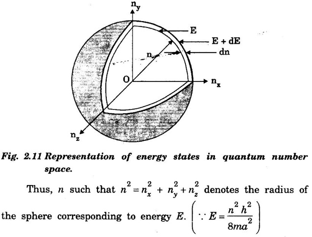
These allowed states form a uniform grid in reciprocal space, or k-space. At $T = 0$ , the fermions fill all the states starting from the origin ( $k = 0$ ) outwards, up to a maximum wavevector magnitude $k_{F}$ , called the Fermi wavevector or Fermi momentum (since $p = ℏ k$ ).

The collection of all occupied states in k-space forms a sphere of radius $k_{F}$ , known as the Fermi sphere. The surface of this sphere, corresponding to the highest energy states, is the Fermi surface. Its energy is precisely the Fermi energy:

E_{F} = \frac{ℏ ^{2} k _{F}^{2}}{2 m}

where $m$ is the mass of the fermion (e.g., the electron effective mass in a solid).

This diagram illustrates the concept of iso-energy surfaces in a 3D quantum number space ($n_x, n_y, n_z$). For a free particle, energy is proportional to $k^2$, so this is equivalent to k-space. The surface of the sphere represents states with the same energy. For a T=0 Fermi gas, all states inside the sphere of radius $k_F$ (the Fermi sphere) are occupied, and the surface itself is the Fermi surface, corresponding to the Fermi energy $E_F$.

The following video provides a more formal discussion, starting from the single-particle Hamiltonian and deriving the quantization of k-space. It then explains how the ground state is constructed by filling these states.

5- Non-interacting electron gas - Course on Quantum Many-Body Physics

This video by Luis Gregorio Dias, from a course on Quantum Many-Body Physics, offers a rigorous treatment of the non-interacting electron gas model, which should align well with your theoretical interests.

First, watch from this timestamp to see how periodic boundary conditions lead to a grid of quantized k-vectors. Then, watch the segment from here, which explains how the N-particle ground state is constructed by filling these k-space states up to the Fermi wavevector, k_F.

4. Calculation of Fermi Energy and Related Quantities

With the concept of the Fermi sphere established, we can now calculate $k_{F}$ and $E_{F}$ as a function of the particle density $n = N / V$ . The total number of particles $N$ is found by summing over all occupied states within the Fermi sphere. In the continuum limit (for large $V$ ), this sum becomes an integral.

The number of states in a small volume $d^{3} k$ of k-space is $V \frac{d ^{3} k}{( 2 π ) ^{3}}$ . For electrons with spin-1/2, each k-state can hold two particles (spin up and spin down), so we have a spin degeneracy factor $g_{s} = 2$ . The total number of particles is therefore:

N = g_{s} \int_{∣ k ∣ \leq k_{F}} \frac{V}{( 2 π ) ^{3}} d^{3} k

The integral is simply the volume of the Fermi sphere, $\frac{4}{3} π k_{F}^{3}$ .

David Tong's lecture notes provide a clear derivation based on the density of states, which is an equivalent and powerful approach.

3. Quantum Gases

These notes provide a concise and rigorous derivation of the Fermi energy.

Please read the section "3.6.2 Degenerate Fermi Gas and the Fermi Surface". The derivation begins by establishing the T=0 step-function distribution, which we have already discussed. Focus on the core calculation that relates the total particle number N to the Fermi energy. Pay close attention to the steps connecting equations (3.41) through (3.43). The text first calculates N by integrating the density of states g(E) up to E_F. It then inverts this relationship to find the final expression for E_F in terms of the particle density n = N/V.

The calculation yields the following fundamental results for a 3D free electron gas:

The Fermi wavevector depends only on the particle density $n = N / V$ :

k_{F} = (3 π^{2} n)^{1/3}

The Fermi energy is then:

E_{F} = \frac{ℏ ^{2} k _{F}^{2}}{2 m} = \frac{ℏ ^{2}}{2 m} (3 π^{2} n)^{2/3}

This shows that the maximum kinetic energy of an electron in the ground state is determined solely by how densely the electrons are packed.

For a rigorous walkthrough of this calculation on a blackboard, the video from the many-body physics course is an excellent resource.

5- Non-interacting electron gas - Course on Quantum Many-Body Physics

This video segment provides a detailed, step-by-step derivation of the Fermi energy.

Watch from this timestamp. The lecturer performs the full calculation of relating the particle number N to the Fermi wavevector k_F and finally to the Fermi energy E_F, showing all the intermediate steps.

Finally, we define the Fermi temperature, $T_{F}$ , as the temperature corresponding to the Fermi energy:

T_{F} = \frac{E _{F}}{k _{B}}

This is not the temperature of the gas. Rather, it is the characteristic temperature scale of the system.

For temperatures $T ≪ T_{F}$ , the gas is said to be degenerate. The system behaves very much like its T=0 ground state, and quantum effects dominate.
For temperatures $T ≫ T_{F}$ , the gas approaches the classical limit.

For electrons in a typical metal, the Fermi energy is of the order of a few electron volts, which corresponds to a Fermi temperature on the order of $1 0^{4}$ to $1 0^{5}$ Kelvin. This is a profound result: it means that even at room temperature ( $\sim 300$ K), the electron gas in a metal is highly degenerate and very far from the classical regime. Its properties are almost entirely determined by the quantum mechanics of its T=0 ground state.

Conclusion

In this lesson, we have laid the groundwork for understanding systems of fermions. We saw how the Pauli exclusion principle forces fermions at zero temperature to fill a "Fermi sphere" in momentum space, leading to a ground state with significant kinetic energy.

Key Takeaways:

The Pauli exclusion principle dictates that identical fermions cannot occupy the same quantum state, leading to the Fermi-Dirac distribution.
At $T = 0$ , the distribution becomes a step function: all states up to the Fermi energy $E_{F}$ are occupied, and all states above it are empty.
In a 3D free electron gas, the Fermi energy and Fermi wavevector are determined by the particle density $n$ : $k_{F} = (3 π^{2} n)^{1/3} and E_{F} = \frac{ℏ ^{2}}{2 m} (3 π^{2} n)^{2/3}$
The Fermi temperature $T_{F} = E_{F} / k_{B}$ is the scale at which thermal energy becomes comparable to the Fermi energy. For $T ≪ T_{F}$ , a Fermi gas is "degenerate".

This T=0 picture is the essential starting point for the theory of metals. In our next lesson, we will build upon this foundation to investigate the properties of an ideal Fermi gas at low, but non-zero, temperatures. We will use the Sommerfeld expansion to calculate the electronic contribution to the heat capacity of metals, a classic result that could not be explained by classical physics.

Recommended resources

1. The Pauli Exclusion Principle and the Fermi-Dirac Distribution

2. The Degenerate Fermi Gas: The Ground State at T=0

3. The Fermi Sphere and Density of States

4. Calculation of Fermi Energy and Related Quantities

Conclusion