Hello! Welcome back to our journey into the foundations of machine learning.
In our last lesson, we saw how gradient descent acts like a relentless navigator, finding the path of steepest descent to minimize a model's loss on the data it was trained on. We celebrated reaching the "bottom of the valley." But this leads to a critical question for any AI architect: if we achieve a near-zero loss on our training data, does that mean we've built a great model? What happens when it encounters new, unseen data in the real world—like a new UPSC aspirant's question or a novel topic for curriculum generation?
Today, we'll tackle this exact challenge. This lesson addresses the learning outcome: Explain the bias-variance tradeoff and its implications for model performance. This is one of the most fundamental concepts in machine learning. Mastering it will allow you to diagnose why models fail and guide your team toward building AI systems that are reliable and generalize well, rather than just being good at memorizing.
1. The Core Problem: Generalization
The ultimate goal of a machine learning model is not to perform perfectly on the data it has already seen, but to generalize its learning to new, unseen data. A model that only memorizes the training data is useless. This is where two sources of error, bias and variance, come into play.
To build an intuition, let's start with an analogy that should resonate with your work in edtech.
The Bias-Variance Tradeoff: Intuition to Diagnosis
This article from Let's Data Science uses a fantastic analogy of two students studying for an exam to introduce bias and variance. It's a great starting point for building a strong mental model.
Please read the first two sections, 'What is the Bias-Variance Tradeoff?' and 'The Analogy: Studying for an Exam'. Focus on the distinction between the 'Slacker' (high bias) and the 'Memorizer' (high variance).
As the analogy illustrates:
- Bias is the error from a model's overly simplistic assumptions. The "slacker" student assumes all answers are "C". This is a simple rule that is wrong most of the time. In machine learning, this leads to underfitting, where the model is too simple to capture the underlying patterns in the data.
- Variance is the error from a model's excessive sensitivity to the training data. The "memorizer" student learns every detail, including typos. This model is too complex and learns the "noise" in the data, not just the "signal." This leads to overfitting, where the model performs well on the training data but fails on new data because the noise is different.
This target practice analogy provides another powerful visual for these concepts.

- Low Bias, Low Variance: The ideal. Predictions are accurate and consistent.
- High Bias, Low Variance: The model is consistently wrong in the same way. (e.g., A linear model trying to fit a curve).
- Low Bias, High Variance: The model's predictions are, on average, centered on the target but are scattered wildly. (e.g., A model that has memorized the training data's noise).
- High Bias, High Variance: The worst case. The model is inaccurate and inconsistent.
2. The Tradeoff: The Push and Pull of Model Complexity
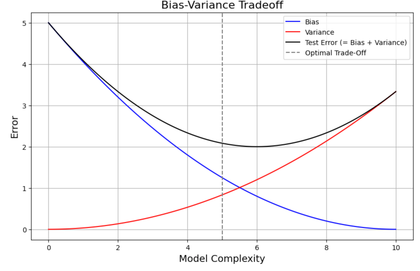
Bias and variance typically have an inverse relationship that is controlled by model complexity.
- Simple Models (e.g., linear regression) are rigid. They make strong assumptions (high bias), but they don't change much if you train them on different subsets of data (low variance).
- Complex Models (e.g., a very deep decision tree or a high-degree polynomial) are highly flexible. They can capture intricate patterns (low bias), but they are also flexible enough to model the random noise in the training data, making them highly sensitive to which data they see (high variance).
This relationship is the "tradeoff": as you decrease bias by making your model more complex, you typically increase its variance, and vice-versa. Your goal as an architect is not to eliminate one or the other, but to find the "sweet spot" of complexity that minimizes the total error.
The graph below is the classic illustration of this concept.
To make this concrete, let's explore a classic example: fitting a polynomial to a set of data points.
What is Bias-Variance Tradeoff?
The following article from IBM provides a clear, illustrated walkthrough of how model complexity (in this case, the degree of a polynomial) affects bias and variance.
Please read the section 'Tradeoff illustrated'. Pay close attention to the three examples: the Degree 1 polynomial (high bias), the Degree 25 polynomial (high variance), and the Degree 4 polynomial (the 'just right' model). Notice how the curve's 'wiggliness' corresponds to its complexity and variance.
This example perfectly demonstrates the tradeoff:
- Underfitting (High Bias): The straight line (degree 1) is too simple. It fails to capture the curve in the data, resulting in high error on both the training points and any future points.
- Overfitting (High Variance): The squiggly line (degree 25) fits the training points almost perfectly, but it has learned the random noise. It would perform very poorly on a new set of points from the same underlying pattern.
- Good Fit (Balanced): The degree 4 polynomial is complex enough to capture the underlying curve (low bias) but not so complex that it memorizes the noise (low variance). It generalizes well.
3. Diagnosing and Fixing the Problem
As an AI architect, you won't be calculating bias and variance directly. Instead, you'll diagnose them by observing model performance on different datasets. You'll need to guide your team on what to do when a model shows symptoms of high bias or high variance.
The Bias-Variance Tradeoff: Intuition to Diagnosis
Let's return to the Let's Data Science article, which provides an excellent 'cheat sheet' for diagnosing these issues and a practical guide for fixing them.
Please read the sections 'What is Bias?', 'What is Variance?', 'How do we detect Bias and Variance?', and 'Practical Guide: Fixing Your Model'. Focus on the table that links symptoms (training/validation error) to a diagnosis (bias/variance) and the clear, actionable steps for fixing each problem.
Here is a summary of the key diagnostic signs and remedies:
| Diagnosis | Symptoms | What to Tell Your Team (The Fix) |
|---|---|---|
| High Bias (Underfitting) | High training error. High test/validation error. |
The model is too simple. 1. Increase model complexity (e.g., try a more powerful architecture like a neural network instead of linear regression). 2. Add more relevant features (feature engineering). 3. Decrease regularization (a technique to penalize complexity, which we will discuss more later). |
| High Variance (Overfitting) | Low training error. High test/validation error. |
The model is too complex or doesn't have enough data. 1. Get more training data (this is often the most effective solution!). 2. Reduce model complexity (e.g., use a smaller network, prune a decision tree). 3. Use regularization to constrain the model. |
Test your understanding!
You are reviewing the performance of a model for your UPSC AI companion that's designed to predict the difficulty of a practice question. Your team reports the following:
- On the 10,000 questions it was trained on, it has a 99% accuracy.
- When you test it on a new set of 1,000 questions, the accuracy drops to 70%.
- What is the most likely problem: high bias or high variance?
- Based on this diagnosis, what is the least likely strategy to help?
a) Get 50,000 more labeled practice questions.
b) Use a simpler model architecture.
c) Train the model for more epochs on the existing data. - What is the most promising strategy?
Show answer
- This is a classic case of high variance (overfitting). The model has clearly memorized the training data (99% accuracy) but fails to generalize to new, unseen data (70% accuracy).
- The least likely strategy to help is (c) Train the model for more epochs on the existing data. This would likely lead to even more overfitting, as the model would have more opportunities to memorize the noise in the training set.
- The most promising strategies would be (a) Get more training data and (b) Use a simpler model architecture (or add regularization). More data is the best cure for high variance, as it makes it harder for the model to find and memorize noise that isn't part of the true signal.
4. The Mathematical Foundation
To complete our first-principles understanding, it's helpful to know that the relationship between these errors can be expressed mathematically. For any given data point, the total expected error of a supervised learning model can be decomposed into three parts:
- Bias²: The error from your model's fundamental assumptions.
- Variance: The error from your model's sensitivity to the specific data it was trained on.
- Irreducible Error: The inherent randomness or "noise" in the data itself. This is a floor on the error that even a perfect model cannot overcome.
You don't need to perform this calculation, but knowing this decomposition exists is key. It proves that there is an unavoidable tradeoff. When you adjust your model's architecture, you are fundamentally trading an increase in one term for a decrease in the other, searching for the point that minimizes their sum.
Conclusion
Today, we've moved from simply training a model to understanding what makes a model good. A low loss on training data is not enough; the true measure of a model is its ability to generalize.
Here are the key takeaways for you as an AI architect:
- Total error is a combination of bias, variance, and irreducible noise.
- Bias (underfitting) comes from models that are too simple. Variance (overfitting) comes from models that are too complex.
- The bias-variance tradeoff means that decreasing one often increases the other. The goal is to find the right level of model complexity to minimize the total error.
- You can diagnose these problems by comparing a model's performance on training data versus unseen test data.
- You can manage the tradeoff by adjusting model complexity, gathering more data, or using techniques like regularization.
You now understand the two principal failure modes of machine learning models. Our next lesson will build directly on this by looking at overfitting and underfitting in more detail, and introducing the practical methodology for diagnosing them: the strategic splitting of data into training, validation, and test sets. This is the standard industry practice for evaluating and tuning the models you will be architecting.