M/M/1 Model Assumptions and Sensitivity Analysis

Welcome back. In our previous lessons, we've explored how to model and optimize queueing systems using the M/M/1 and M/M/s models. We saw, for instance, the dramatic reduction in waiting time at your boudoir photoshoot—from 48 minutes to just over 2 minutes—by simply adding an assistant. These models are powerful, but their power comes from a set of very specific, and sometimes restrictive, assumptions.

Today, we will turn a critical eye on those foundations. Your learning outcome is to: Critically evaluate the assumptions of the M/M/1 model for both the photoshoot and intimacy scenarios, and analyze the sensitivity of outcomes to violations of these assumptions. As an experienced statistician and optimizer, you know that understanding a model's limitations is just as crucial as knowing its applications. This lesson is about moving from "how to use the model" to "when to trust the model."

Deconstructing the M/M/1 Model: A Foundation of "M"s

The Kendall notation M/M/1 is a compact descriptor for a model built on three core pillars, each representing a significant assumption about the system's behavior. Let's dissect them one by one.

The First "M": Markovian Arrivals (The Poisson Process)

This assumption states that arrivals to the system follow a Poisson process. As you know from your background in stochastic processes, this implies three key properties:

Independence: The arrival of one "customer" is independent of all others.
One at a time: Customers arrive individually, not in batches.
Constant Rate: The average arrival rate, $λ$ , is constant over time.

A fundamental consequence of these properties is that the time between arrivals is exponentially distributed, which gives the process its "memoryless" nature. The time until the next arrival is completely independent of when the last one occurred.

Queuing theory and Poisson process

This video provides an excellent intuitive and mathematical walkthrough of the Poisson process and its assumptions.

First, watch the segment that explains how customer arrivals are modeled as a Poisson process, starting from the idea of independent events. Then, watch the brief introduction to the unrealistic model, which highlights the core assumptions.

Critique for Your Scenarios:

Boudoir Photoshoot: Is the arrival of "styled looks" ready for photography a Poisson process?
- Independence & Constant Rate: Probably not. The time to prepare a complex look might delay the start of the next. Creative energy might lead to a burst of quick looks early on, followed by a slowdown due to fatigue. This suggests a time-varying and state-dependent arrival rate, violating the constant rate and independence assumptions. The document "QUEUEING THEORY AND MODELING" discusses the issue of time-varying demand and how it can make steady-state models inappropriate.
Hotwife Intimacy: Is the arrival of "opportunities for an encounter" (driven by desire or availability) a Poisson process?
- Independence: Highly unlikely. The desire for a new encounter is almost certainly influenced by the timing and quality of the last one, directly violating the memoryless property.
- Constant Rate: Availability and desire fluctuate based on work schedules, energy levels, and emotional states, so the rate $λ$ is far from constant.

The Second "M": Markovian Service Times (The Exponential Distribution)

This is perhaps the most scrutinized assumption. It posits that service times follow an exponential distribution. Like the arrival process, this implies service is memoryless: the remaining time to complete a service is independent of how long it has already taken. A key, and often unrealistic, feature of the exponential distribution is that its mode is at zero, meaning very short service times are the most probable.

Chapter 2 Basics of Queueing Theory | Simio and Simulation

This chapter from the Simio and Simulation textbook provides a clear-eyed comparison of queueing theory and simulation, directly addressing the realism of assumptions.

Please read the section titled Queueing Theory vs. Simulation. Pay close attention to the critique of assuming exponential service times.

Critique for Your Scenarios:

Boudoir Photoshoot: Is the time to photograph a look exponentially distributed?
- This seems very improbable. A photoshoot has a natural overhead—adjusting lighting, directing the pose—which establishes a practical minimum duration. The idea that a zero-second shoot is the most likely outcome is nonsensical. A distribution with a non-zero mode, like a Normal, Log-Normal, or even a simple Uniform distribution, would likely be more realistic.
Hotwife Intimacy: Are encounter durations exponential?
- Again, this is highly unrealistic for similar reasons. Encounters have a natural rhythm and duration, making a mode of zero absurd.

Other Implicit Assumptions

Beyond the two "M"s, the basic model carries other assumptions.

Waiting Line Models: Single Server - 6 - M/M/1, M/G/1 and M/D/1 (Part 1/2)

This video clearly lists the underlying assumptions of the M/M/1 model that often go unstated.

Watch the segment from discussing the other assumptions. The presenter covers the infinite calling population, infinite queue size, FCFS discipline, and infinitely patient customers.

Let's evaluate these:

Infinite Queue Size: The model assumes an infinite waiting room. In the photoshoot, the number of "looks" is finite. In the intimacy scenario, the "queue" of desired encounters is also finite.
FCFS (First-Come, First-Served): In a photoshoot, you might prioritize a particularly stunning outfit-pose combination. In the intimacy context, scheduling is a negotiation, not a strict queue. Priority queue models, as mentioned in the "QUEUEING THEORY AND MODELING" resource, would be more appropriate.
No Reneging (Customers are infinitely patient): If a photoshoot look waits too long, the model or stylist might lose enthusiasm (reneging). If an intimacy opportunity is delayed, desire may wane (balking or reneging).

The Impact of Variability: Sensitivity Analysis with M/G/1

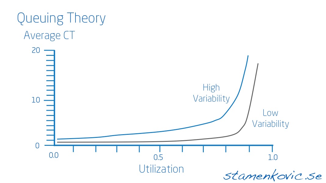
So, the M/M/1 assumptions are often violated. But by how much does it matter? The most significant factor is variability. The M/M/1 model, with its exponential distributions, assumes a high degree of randomness. The coefficient of variation (CV), which is the ratio of the standard deviation to the mean ( $C V = σ / mean$ ), is the key metric here. For an exponential distribution, $C V = 1$ .

What happens when service times are not exponential? We can use the M/G/1 model, which assumes Poisson arrivals but allows for a General service time distribution. The formula for the average wait in the queue, known as the Pollaczek-Khinchine formula, provides the answer.

QUEUEING THEORY AND MODELING

This section of the Columbia Business School paper is crucial. It introduces models that relax the exponential assumption and shows exactly how variability impacts waiting time.

Please read the section titled The M/G/1 and G/G/s models. Focus on equation (6) for the M/G/1 system and equation (7), the approximation for the G/G/s system. The key insight is how the CV^2 terms for both service and arrival times directly influence the average delay.

The M/G/1 formula for average wait time ( $W_{q}$ ) can be elegantly expressed in relation to the M/M/1 wait time:

W_{q, M/G/1} = W_{q, M/M/1} \times (\frac{1 + C V _{s}^{2}}{2})

Here, $C V_{s}$ is the coefficient of variation of the service time. This equation is a powerful tool for sensitivity analysis:

Case 1: Exponential Service (M/M/1). Here, $C V_{s} = 1$ . The adjustment factor is $(1 + 1^{2}) /2 = 1$ . The formula reduces to the M/M/1 case, as expected.
Case 2: Constant Service (M/D/1). If your process is perfectly consistent and every service takes the exact same amount of time ( $D$ for deterministic), then the standard deviation is 0, so $C V_{s} = 0$ . The factor becomes $(1 + 0^{2}) /2 = 0.5$ . Wait time is cut in half compared to the M/M/1 model, just by eliminating variability!
Case 3: Low-Variability Service. If service times are fairly consistent, like a uniform or normal distribution, $C V_{s} < 1$ . The factor will be less than 1, resulting in shorter waits than predicted by M/M/1.
Case 4: High-Variability Service. If service times are erratic (a mix of very short and very long), then $C V_{s} > 1$ . The factor is greater than 1, and waiting times will be even worse than the M/M/1 prediction.

This relationship is vividly illustrated in the following graph.

This graph shows how average cycle time (CT), which includes wait time, increases with utilization. Note how the "High Variability" curve (analogous to M/M/1 with CV=1) is significantly steeper and higher than the "Low Variability" curve (analogous to M/G/1 with CV<1).

Application: Optimizing by Reducing Variability

Let's apply this to your photoshoot scenario, using the parameters from our M/M/1 analysis: $λ = 4$ looks/hr, $μ = 5$ looks/hr, $ρ = 0.8$ , and $W_{q, M / M /1} = 48$ minutes.

M/M/1 Prediction (High Variability): 48 minutes wait.
M/D/1 Prediction (Zero Variability): What if you could standardize the shooting process so each look takes exactly 12 minutes? The wait time would become $W_{q} = 48 \times 0.5 = 24$ minutes. You've halved the waiting time without making the photographer shoot any faster on average. For an efficiency expert, this is a profound insight: reducing variance can be as effective as increasing the mean service rate.
Intimacy Scenario: The same logic holds. If the duration of encounters becomes more predictable ( $C V_{s} < 1$ ), the "waiting time" (periods of unfulfilled desire when both partners are theoretically free) will decrease, leading to higher overall satisfaction.

The approximation for the G/G/s model, $W_{q} \approx W_{q, M / M / s} \times \frac{C V _{a}^{2} + C V _{s}^{2}}{2}$ , further generalizes this, showing that reducing variability in either the arrival process or the service process will reduce congestion.

Conclusion

Today we've moved beyond the simple application of queueing formulas to a more sophisticated analysis of their validity. You now have a framework for critically assessing the M/M/1 model and quantifying the impact of its assumptions.

Key Takeaways:

The M/M/1 model's assumptions (Poisson arrivals, exponential service, FCFS, etc.) represent a state of high, memoryless randomness.
These assumptions are often unrealistic for real-world processes like photoshoots or personal intimacy, which exhibit memory, time-varying rates, and non-zero-mode service times.
The M/G/1 model allows us to quantify the impact of service time variability. The key insight is that waiting time is highly sensitive to the coefficient of variation ( $C V_{s}$ ) of the service process.
Reducing variability ( $C V_{s} < 1$ ) can dramatically reduce waiting times, often more easily than increasing the average service rate. The M/M/1 model, which assumes $C V_{s} = 1$ , frequently provides an upper-bound or pessimistic estimate for systems with more controlled processes.

In our next module, we will shift our focus from managing flows and availability to managing resources with Inventory Models. We'll start by applying ABC Analysis to prioritize both lingerie pieces for the photoshoot and intimacy-building activities in the hotwife scenario.

Recommended resources