Welcome to our second lesson on Queueing Theory. In our previous session, we established Little's Law as a powerful descriptive tool, allowing us to diagnose the state of a system by relating the average number of items (), the arrival rate (), and the average time spent in the system (). We saw how observing a buildup of work-in-progress and an increase in lead time points directly to a bottleneck.
Today, we shift from description to prediction. We will explore one of the most fundamental predictive models in queueing theory. Your learning outcome for this lesson is to: Use the M/M/1 model to predict wait times for outfit-pose setups with a single photographer and to analyze the impact of encounter duration variability on the hotwife's 'wait' for the bull's availability. This will equip you not just to measure a queue, but to forecast its behavior and understand the deep-seated drivers of waiting.
From Description to Prediction: The M/M/1 Model
The M/M/1 model is a cornerstone of queueing theory that allows us to calculate expected wait times and queue lengths based on two key parameters: the rate of arrivals and the rate of service. To understand the model, we first need to decipher its name, which comes from a standard classification system called Kendall's Notation.
This section from a lecture on queueing models introduces the standard notation used to describe queueing systems.
Please read the brief section on Kendall Notation (A/B/c/N/K). Focus on understanding what each component represents, particularly the first three: A, B, and c. Note the definition of 'M' as Markovian, signifying an exponential distribution. This will clarify why M/M/1 has its name.
As you've just read, the M/M/1 notation specifies:
- M (Arrival Process): Arrivals are Markovian, meaning they follow a Poisson process. The time between consecutive arrivals is exponentially distributed. This implies that arrivals are random and independent; an arrival occurring now gives no information about when the next one will happen.
- M (Service Process): Service times are also Markovian, or exponentially distributed. This implies a "memoryless" property: the time already spent servicing a customer doesn't affect the remaining service time. This is a strong assumption, implying high variability where some services are very quick and others take a very long time.
- 1 (Number of Servers): There is a single server handling the queue.
For this system to be stable and for queues not to grow infinitely, there is a crucial condition: the average arrival rate, denoted by , must be less than the average service rate, denoted by .
This makes intuitive sense: if customers arrive faster than they can be served, the line will grow without bound.
Utilization and the Onset of Congestion
A critical metric derived from and is the server utilization factor, (rho).
Utilization represents the proportion of time the server is busy. While a high might seem efficient, it is also a direct indicator of system congestion. As approaches 1 (or 100%), the system comes under immense pressure, and waiting times begin to increase dramatically. This relationship is not linear; the pain of waiting grows exponentially as utilization nears its limit.
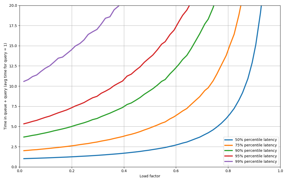
The video below offers a clear, practical explanation of the M/M/1 model's core formulas and the intuition behind them.
13a Queuing Model essence, arival & service rate, 8 formulae
This video provides a concise lecture on the essential components and formulas of the M/M/1 queuing model.
Please watch the following segments: First, understand the definitions of arrival rate (\lambda) and service rate (\mu) and the critical importance of the stability condition (\mu > \lambda). Next, review the description of the distributions for arrivals (Poisson) and service (negative exponential). Finally, carefully review the eight operating characteristic formulas. Pay closest attention to the formulas for L (average number in system), L_q (average number in queue), W (average time in system), and especially W_q (average time in queue).
To summarize the key predictive formulas for a stable M/M/1 system:
| Performance Metric | Formula | Alternative Form |
|---|---|---|
| Server Utilization () | ||
| Avg. Time in System () | ||
| Avg. Time in Queue () | ||
| Avg. Number in System () | ||
| Avg. Number in Queue () |
Note that these formulas are consistent with Little's Law, which you learned in the previous lesson: and .
Application 1: Predicting Wait Times in a Boudoir Photoshoot
Let's model the boudoir photoshoot workflow. The single photographer is our server, and the distinct outfit-pose combinations ("looks") are the customers arriving to be shot.
System Parameters:
- Arrival Rate (): Based on styling and preparation, new looks become ready to be photographed at an average rate of 4 looks per hour.
- Service Rate (): The photographer, when working continuously, can complete an average of 5 looks per hour.
Analysis:
First, we check for stability: . The system is stable.
Next, we calculate the photographer's utilization:
This means the photographer is expected to be busy 80% of the time. Now we can predict the average waiting time for a look. We are interested in the time a look spends waiting after it's ready but before shooting begins. This is .
Converting to minutes: .
We can also predict the total time a look will spend in the system, from the moment it's ready until the shot is final ():
This is consistent, as the total time () is the waiting time () plus the service time ( hours, or 12 minutes): minutes.
Prediction: Under these conditions, the M/M/1 model predicts that a styled look will wait, on average, 48 minutes before the photographer even starts shooting it. This quantifies the delay caused by operating at 80% utilization.
Application 2: The Impact of Encounter Duration Variability
Now, let's model the hotwife's encounters with her bull. The bull is the single server, and the hotwife's desires for specific encounters are the customers. Your goal is to analyze the impact of encounter duration variability.
This is where your background as a statistician becomes particularly useful. The "M" for service in the M/M/1 model assumes exponential service times. A key property of the exponential distribution is that its standard deviation is equal to its mean. This corresponds to a coefficient of variation () of 1, which represents high variability.
To analyze the impact of variability, we can compare the M/M/1 result () to a scenario with lower variability, using a more general formula from the M/G/1 model (where 'G' stands for a general service distribution).
This resource discusses how both utilization and service time variability affect queue performance.
Focus on the section "Effect of Utilization and Service Variability". Pay close attention to the definition of the coefficient of variation (cv) and the formula for L_Q in an M/G/1 queue. Notice how it separates the M/M/1 part from a term that depends on cv. This is the key to our analysis.
The Pollaczek-Khinchine formula for the average number of customers in the queue for an M/G/1 system can be written as:
And since , this allows us to see how wait time changes with variability ().
System Parameters:
- Arrival Rate (): The hotwife has, on average, 1 new desire for an encounter per week.
- Service Rate (): The bull can, on average, fulfill 1.25 encounters per week. (This means an average "service time" of weeks).
The system is stable () and the utilization is .
Scenario A: High Variability (M/M/1 Model)
The encounters are spontaneous and unpredictable in duration. We model this with an exponential distribution, so .
With high variability, the average wait from when a desire forms until the encounter can be planned and started is 3.2 weeks.
Scenario B: Lower Variability
The hotwife and bull structure their time to make encounter durations more consistent. The average duration is the same, but the variability is lower. Let's assume the standard deviation is now only half the mean, giving .
Analysis: By reducing the variability of the "service time" (making encounter durations more predictable), while keeping the average duration and arrival rate constant, the predicted waiting time for an encounter drops from 3.2 weeks to 2.0 weeks—a reduction of nearly 40%. This demonstrates a profound principle of queue management: variability is a major cause of waiting. For a given level of utilization, a more consistent and predictable system will always have shorter queues.
Conclusion
In this lesson, we advanced from the descriptive power of Little's Law to the predictive capabilities of the M/M/1 model. We have seen how this model, built on specific assumptions about random arrivals and service times, allows us to forecast key performance metrics like waiting time.
Key Takeaways:
- The M/M/1 model describes a single-server queue with Poisson arrivals and exponential service times.
- It requires the arrival rate to be less than the service rate () for the system to be stable.
- The utilization factor () is a critical driver of congestion. As approaches 1, waiting times increase non-linearly.
- The model's formulas can predict average wait times () and queue lengths (), providing a quantitative basis for decision-making.
- A crucial insight, especially for an optimizer, is that reducing service time variability () can dramatically decrease waiting times, even if the average service rate remains unchanged.
In our next lesson, we will extend this analysis to systems with more than one server. We will explore the M/M/s model to evaluate the benefits of adding capacity, such as bringing an assistant to the photoshoot, and see how parallel processing changes the dynamics of the queue.