Optimizing Hotwife Encounters with Little's Law

The Fundamental Relationship: Unpacking Little's Law

At its heart, Little's Law connects three fundamental measures of a process. A great way to start is by familiarizing yourself with these core concepts and the law that binds them.

The law establishes a deterministic relationship between these three averages. Knowing any two allows you to calculate the third. The variables are often denoted differently depending on the context, so you will see $I=R\times T$ used interchangeably with $L=\lambda \times W$, where:

• $L$ is the average number of items in the system (Inventory).
• $\lambda$ (lambda) is the average arrival/throughput rate (Throughput).
• $W$ is the average time an item spends in the system (Wait/Lead Time).

For the remainder of this lesson, we will use the $L=\lambda W$ notation.

The Power of Simplicity: Why Little's Law is So Robust

Given your background in statistics and modeling, you are accustomed to carefully scrutinizing the assumptions behind any formula. Little's Law is remarkable precisely because its assumptions are so minimal, making it applicable in a vast range of real-world scenarios.

While these assumptions appear straightforward, the law's true power lies in what it doesn't require. To appreciate this, we'll turn to the foundational paper by John Little himself, written 50 years after he first published his proof.

The key takeaway is that Little's Law is not a statistical approximation; it is an algebraic identity for the averages of any stable process. This robustness allows us to apply it with confidence to messy, real-world systems that don't fit the clean assumptions of many other queueing models.

From Law to Diagnosis: Identifying Bottlenecks

So, how does this simple law help us find a bottleneck? A bottleneck is the stage in a process that has the lowest capacity. It governs the maximum possible throughput ($\lambda$) for the entire system. Any attempt to push work through the system faster than the bottleneck can handle it is futile.

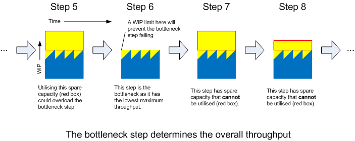
When work arrives at a bottleneck faster than it can be processed, a queue forms. This is where Little's Law becomes a diagnostic tool. Let's re-arrange the formula:

If the throughput $\lambda$ is capped by a bottleneck, and the amount of Work-In-Progress $L$ before that bottleneck increases, the average waiting time $W$ must necessarily increase. Therefore, the two primary symptoms of a bottleneck are:

1. A growing queue or a consistently large amount of Work-In-Progress (WIP), our $L$, before a specific process step.
2. An increasing Lead Time, our $W$, for items moving through the process.

The following reading explains this connection in practical business terms.

Now, armed with this framework, let's apply it to your specific scenarios.

Application 1: The Boudoir Photoshoot Workflow

Imagine a photoshoot session designed to produce a set of 12 distinct "looks" (outfit-pose combinations). The workflow consists of three main stages: Makeup & Styling, Set Preparation, and Shooting.

• System: The entire process from the start of styling for the first look to the final capture of the last look.
• Items: The "looks" or setups.
• Metrics:
  • Throughput ($\lambda$): The rate at which completed looks are finalized. Let's say the goal is 3 looks per hour.
  • Work-In-Progress ($L$): The number of looks that are "in the system." This can be defined as looks that have been styled but are not yet fully shot.
  • Lead Time ($W$): The average time a single look spends in the system, from the moment styling begins until its final shot is captured.

Diagnosing the Bottleneck:

Let's assume the photographer is extremely meticulous and takes a long time to perfect the lighting and composition for each shot. The stylist, however, works quickly.

1. Observation: We notice that the model is often fully styled and waiting. We might have two looks fully styled and prepped (one on the model, one on a mannequin), but the photographer is still working on the previous one. The WIP ($L$) of "ready-to-shoot" looks is consistently high. Let's say, on average, $L=2$ looks are always in a queue waiting for the photographer.
2. Measurement: We track the output over a 4-hour session and find that only 8 looks were completed. The system's actual Throughput ($\lambda$) is $8\text{ looks}/4\text{ hours}=2$ looks per hour, not the planned 3. The photographer's capacity is the system's constraint.
3. Diagnosis with Little's Law: We can now calculate the average lead time for a look: $$W=\frac{L}{\lambda }=\frac{2\text{ looks in queue}}{2\text{ looks/hour}}=1\text{ hour}$$ This means that, on average, from the moment a look is selected for styling, it takes a full hour before it's "done." If the actual styling and shooting time for one look is only 25 minutes, this implies an average of 35 minutes is pure waiting time, spent in the queue before the photographer. The high WIP and long lead time, coupled with the low throughput, definitively point to the Shooting stage as the bottleneck.

Application 2: The "Queue" of Desired Encounters

This application is more abstract but follows the exact same logic. We model the hotwife's desires for intimacy with her bull as items entering a system.

• System: The process of realizing desired intimate encounters.
• Items: Distinct "desired encounters" (e.g., a specific fantasy, a weekend trip, a type of date night).
• Metrics:
  • Throughput ($\lambda$): The "fulfillment rate." The average number of desired encounters that are successfully actualized per month.
  • Work-In-Progress ($L$): The "backlog of desire." The average number of distinct, unfulfilled desires in her mental queue at any given time.
  • Lead Time ($W$): The "desire-to-fulfillment" time. The average time from when a desire is formed until the encounter happens.

Diagnosing the Bottleneck:

Suppose the hotwife is creative and constantly thinks of new encounter ideas, but her bull has a demanding job and limited availability.

1. Observation: The hotwife keeps a mental or physical list of ideas she wants to explore. This list seems to grow faster than items are checked off. At any given time, she has about 12 specific ideas she's waiting to act on. Her WIP ($L$) is, on average, 12 desires.
2. Measurement: Looking back over the past six months, they have managed to have 9 of the encounters from her list. The system's Throughput ($\lambda$) is $9\text{ encounters}/6\text{ months}=1.5$ encounters per month. This rate is governed by the bull's availability.
3. Diagnosis with Little's Law: We calculate the average time it takes for one of her desires to become a reality: $$W=\frac{L}{\lambda }=\frac{12\text{ desired encounters}}{1.5\text{ encounters/month}}=8\text{ months}$$ The diagnosis is stark. An idea she has today will, on average, take 8 months to be fulfilled. This quantifies the feeling of a slow-moving or stagnant dynamic. The bottleneck is not her rate of desire or planning effort; it is unequivocally the bull's availability, which caps the system's throughput. The large backlog of desire ($L$) and the resulting long lead time ($W$) are direct symptoms of this constraint.

Conclusion

In this lesson, we have explored the elegant and powerful nature of Little's Law. It provides a fundamental equation, $L=\lambda W$, that connects the average inventory, throughput, and lead time of any stable system. Its strength lies in its robustness, holding true regardless of statistical distributions or queueing disciplines. This makes it an invaluable "first-principles" tool for process analysis.

Key Takeaways:

• Little's Law is a fundamental identity: It relates the three core performance measures of any flow process: Work-In-Progress (Inventory), Throughput, and Lead Time.
• It is surprisingly robust: It applies to non-stationary processes and is independent of service order, making it ideal for real-world diagnosis.
• It is a powerful bottleneck diagnostic: By measuring throughput ($\lambda$) and observing where work-in-progress ($L$) accumulates, you can calculate the impact on lead time ($W$) and pinpoint the constraints in your system.

We have applied this law to diagnose bottlenecks in both a tangible workflow (the photoshoot) and an intangible queue (the fulfillment of desires), demonstrating its versatility.

In our next lesson, we will build upon this foundation. While Little's Law is descriptive—it tells you what your system is doing—we will move into predictive modeling with the M/M/1 model. This will allow us to analyze how a system will behave under different conditions, predicting specific wait times and queue lengths based on the statistical properties of arrivals and service.