Welcome back. In our last lesson, we explored the crucial difference between assets that deteriorate gradually and those that fail suddenly, establishing that the failure mode dictates the optimal maintenance and replacement strategy. You learned to distinguish between a wear-out process () and a random failure process (), which forms the foundation for today's analysis.
Today, we will build the specific policy for the first case. Your learning outcome is to apply an Individual Replacement Policy to determine the optimal time to replace a key lingerie piece based on its cost and declining effectiveness. This involves a clear-eyed economic analysis, where we trade off the initial cost of an asset against its rising operating and maintenance costs over time. We will transform the abstract concept of "deterioration" into a concrete, quantifiable decision rule.
The Economics of Deterioration
When an asset deteriorates, it doesn't just get older; it becomes more expensive to keep. This expense isn't always about direct repairs. It can be an implicit cost, such as lower efficiency, poorer quality output, or, in our photoshoot scenario, declining aesthetic appeal. The Individual Replacement Policy addresses this by seeking the "sweet spot"—the replacement age that minimizes the total cost averaged over the asset's life.
A powerful way to visualize this is the P-F Curve, which plots an asset's condition against time.
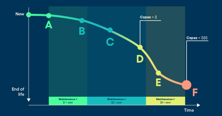
As the curve shows, an asset's condition degrades, and the cost of maintaining its performance (the "Maintenance $" bars) rises. We replace the asset not when it fails completely (point F), but when it becomes more economical to buy a new one than to continue paying the increasing costs of the old one.
Determining the Economic Life of an Asset
To find this optimal replacement point, we need to track two primary types of costs:
- Capital Cost: The initial purchase price of the asset, spread out over its life.
- Operating & Maintenance (O&M) Costs: These are the costs that increase as the asset ages.
The average total cost per period will initially decrease as the capital cost is spread over more periods, but it will eventually rise as the escalating O&M costs begin to dominate. The point where the average total cost is at its minimum defines the asset's economic life.
The following presentation provides a clear, step-by-step method for calculating this economic life.
Replacement and Maintenance Analysis | PDF - Slideshare
This presentation visually breaks down the calculation of an asset's economic life. It clearly separates capital costs from operating costs and shows how they combine to reveal the optimal replacement point.
Please review the slides from the start of section 1.4. Pay close attention to Figure 1.2, which illustrates the relationship between capital recovery cost, O&M cost, and total cost. Then, carefully follow the logic in Table 1.1 for the interest-free case (i=0%). Notice how the "Average Total Cost" (Column F) is calculated and how its minimum value determines the economic life.
Application: Optimizing the Lingerie Wardrobe
Let's apply this method to our primary scenario: determining the optimal time to replace a signature lingerie piece for your boudoir photoshoots.
Here's how we define our costs:
- Capital Cost (C): The purchase price of the high-end lingerie piece. Let's assume C = $400.
- Scrap Value (S): We'll assume the piece has no resale value, so S = $0.
- Operating & Maintenance Cost, : This is the crucial variable. It represents the "cost" of the piece's declining effectiveness (its "sexiness") for the -th photoshoot. This cost can be viewed as the value of the extra effort needed to compensate for the wear—more intricate lighting, longer post-processing time, or simply the opportunity cost of a less impactful final image. Let's model this as an increasing function. Suppose the cost is negligible for the first use but increases by $30 for each subsequent use.
- ...and so on.
Now, we can construct a table just like the one in the presentation to find the optimal number of uses. The goal is to find the number of uses, , that minimizes the average cost per use, .
Let's calculate it:
| (1) Use (n) | (2) O&M Cost for this Use, | (3) Cumulative O&M Cost, | (4) Total Cost, | (5) Avg. Cost per Use, |
|---|---|---|---|---|
| 1 | $0 | $0 | $400 | $400.00 |
| 2 | $30 | $30 | $430 | $215.00 |
| 3 | $60 | $90 | $490 | $163.33 |
| 4 | $90 | $180 | $580 | $145.00 |
| 5 | $120 | $300 | $700 | $140.00 |
| 6 | $150 | $450 | $850 | $141.67 |
The analysis is clear. The average cost per use decreases, reaching a minimum of $140.00 at the 5th use. After that, the rapidly increasing O&M cost makes the average cost begin to climb again. Therefore, the economic life of this lingerie piece is 5 uses. To operate most economically, you should plan to replace it after the 5th photoshoot.
The Formal Replacement Rule
Another way to express this is through a simple decision rule. The "Replacement Problem" PDF resource provides the formal mathematical justification.
This document provides the classic Operations Research formulation for the individual replacement problem.
Please read the section Replacement of Equipment that Deteriorates Gradually. This section formalizes the logic we just applied. The key takeaway is the replacement rule derived at the end: you should replace an item if the operating cost in the next period is greater than the average total cost in the current period. Then, quickly review the first sample problem (1801) to see this rule applied in a tabular format.
The rule states: Replace the asset at the end of period if .
Let's check this with our lingerie example:
- At the end of use 4: The cost of the next use is . The average cost is . Since , we keep the item.
- At the end of use 5: The cost of the next use is . The average cost is . Since , the rule tells us to replace the item.
Both methods—finding the minimum average cost and applying the period-over-period rule—lead to the same conclusion: the optimal replacement point is after 5 uses.
Conceptual Application: "Replacing" an Intimacy Dynamic
This model, while designed for physical assets, can also be a powerful conceptual tool for the hotwife-bull intimacy scenario. Here, you are not replacing a person, but rather "replacing" a routine or a specific dynamic of the relationship that has begun to deteriorate.
- The "Asset": The current established pattern of encounters—the type of activities, the communication style, the scheduling method.
- Capital Cost (C): The initial emotional, logistical, and communicative investment made by the hotwife to establish this particular dynamic with her bull.
- Deterioration: The dynamic loses its novelty and excitement. The same activities yield less satisfaction than they used to.
- O&M Cost, : The increasing emotional labor or planning effort required to achieve the desired level of satisfaction from the now-stale dynamic. It's the "work" needed to make the old routine feel fresh again.
- Replacement: This means making a conscious, deliberate change to the dynamic. It's a "reset"—introducing new types of encounters, changing the rules of engagement, or having a deep conversation to redefine goals and expectations. This "new asset" comes with its own "capital cost" (the effort of the reset).
The individual replacement model provides a framework for the hotwife to decide when a full "reset" is more effective than continuing to patch the old dynamic. The model suggests that the time for a reset is when the effort required to make the next encounter within the old dynamic satisfying () feels greater than the average satisfaction-per-unit-of-effort she has experienced with that dynamic so far (). It provides a logical trigger for proactive relationship management, moving beyond simply reacting to dissatisfaction.
Conclusion
In this lesson, we have moved from theory to practice by applying the individual replacement policy to an asset with gradual deterioration. You have learned how to calculate the economic life of an asset by finding the point where its average cost per period is minimized.
Key Takeaways:
- The Individual Replacement Policy is an economic model used for assets whose operating costs increase over time.
- The optimal replacement time, or economic life, is the point that minimizes the average total cost per period.
- This can be found by creating a table that tracks cumulative costs or by using the rule: Replace when the next period's operating cost exceeds the current average cost.
- The concept of "cost" can be abstract and include factors like declining aesthetic value, loss of effectiveness, or increased emotional labor.
In our next lesson, we will shift our focus. Having mastered individual replacement for deteriorating items, we will investigate the Group Replacement Policy, a strategy typically used for large numbers of items that fail suddenly. We will see how this can be applied to refreshing photoshoot accessories and evaluating periodic joint 'reset' conversations with partners.